Riemann Sum and Integral Explorer
Watch rectangles converge on an integral, and see why the midpoint and Simpson rules beat endpoint sums at the same strip count.
Simulator
- Approximation Left endpoint rule with 1 strips.
- 0
- Exact value Hand integrated, so the error beside it is a real error.
- 2.66667
- Error Signed. Positive means this rule overestimates.
- -2.667
- Strips
- 1
- Strip width Called h. Every rule’s error is a power of it.
- 2
- Measured order Doubling the strips divides the error by 2 to this power. Theory says 1.
- 0.862
Each rectangle takes its height from its left edge, so it undershoots a rising curve.
Rising throughout, so the left sum is below the answer and the right sum above it.
- Left endpoint
- Right endpoint
- Midpoint
- Trapezoid
- Simpson
Citing this tool
Last updated . Add the date you accessed it as well, which a citation of a page that can change asks for. If a specific result matters, cite the permalink from the tool’s share row instead of this page: it reproduces the exact parameters.
The equation
Riemann, Habilitationsschrift (1854)
The definition, not the shortcut
An integral is defined as a limit of sums. Most people meet that definition once, accept it, and then replace it permanently with a table of antiderivatives. That works, and it leaves the original idea as a piece of formal scaffolding rather than something you can picture.
So here the sum is the object on screen and the exact value is the thing it approaches. Turn the strips up and watch the error column, not the picture: the rectangles stop looking different long before the error stops shrinking, which is itself worth noticing.
Why left and right sums bracket the answer, until they do not
On a rising curve every left rectangle sits under the graph and every right one pokes above it, so the true value is trapped between the two sums. That is a genuinely useful guarantee, and it is easy to over-generalise.
Select sin x on [0, π] and it collapses. The two
sums come out identical, and both are too small. The reason is that
bracketing was never a property of the method, it was a property of the
function being monotonic. Once the curve rises and then falls, the
undershoot on the way up is paid for by an overshoot on the way down, and
the guarantee evaporates.
Order of accuracy is the thing that actually matters
The five rules do not just differ in how accurate they are, they differ in how fast they improve. That distinction is the whole subject:
| Rule | Order | Error becomes |
|---|---|---|
| Left or right endpoint | 1 | half |
| Midpoint | 2 | a quarter |
| Trapezoid | 2 | a quarter |
| Simpson | 4 | a sixteenth |
The measured order readout computes this live by doubling the strip count and comparing errors, so you are not taking the table on trust. It also explains the error plot, which is drawn on a linear scale: every line falls towards zero as the strips increase, and the higher a rule’s order, the sooner its line flattens onto the axis.
Midpoint and trapezoid: same order, opposite errors
The midpoint rule takes the height from the centre of each strip, so the slice of curve above the rectangle on one side roughly cancels the slice below it on the other. The trapezoid rule instead joins the two endpoints with a straight line, which turns out to be exactly the average of the left and right sums. Worth verifying on screen.
Both are second order, and for a curve bending upwards they err in opposite directions: the trapezoid overestimates, the midpoint underestimates by about half as much. That two-to-one relationship is not a coincidence. Combining them in that ratio to cancel the leading error is precisely how Simpson’s rule is derived.
Why Simpson’s rule is exact for a cubic
Simpson fits a parabola through each pair of strips. Its error term depends on the fourth derivative of the function, and a cubic’s fourth derivative is zero everywhere, so the error is not merely small, it is zero.
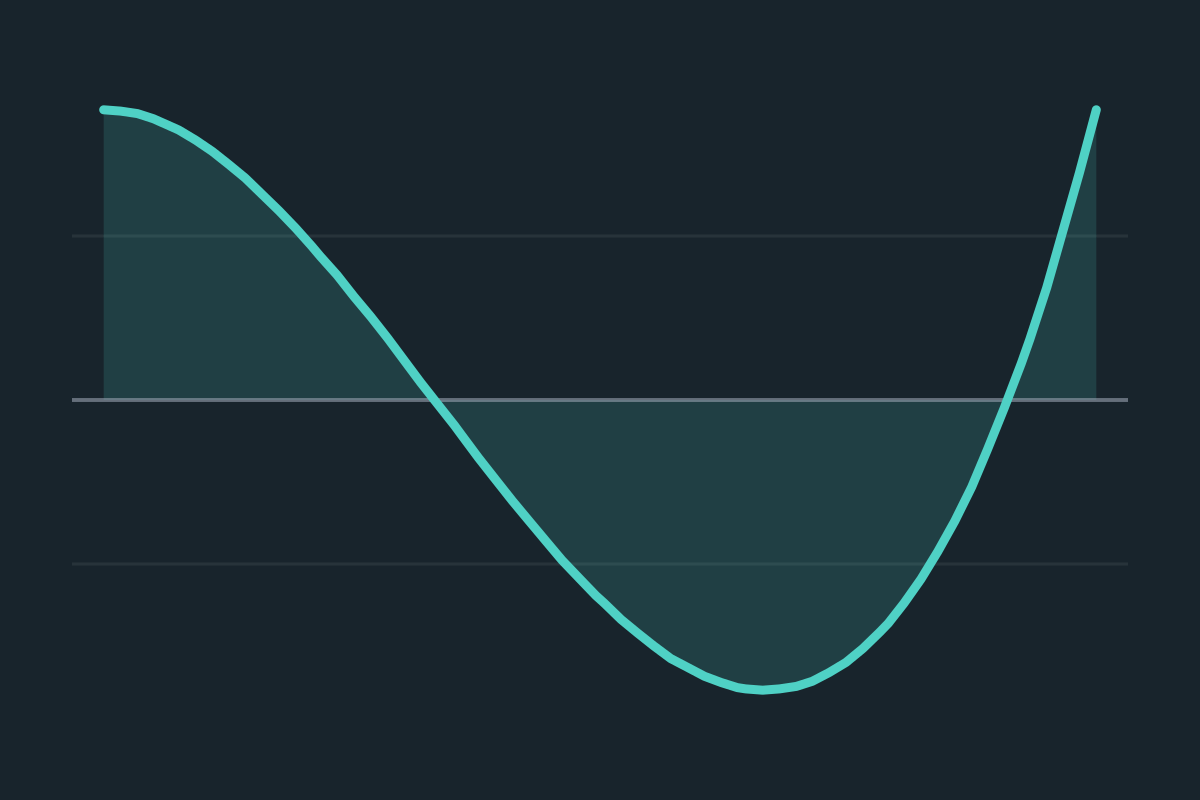
Choose x³ - 3x and set the strips to two. Simpson reports
-0.75, the exact answer, from a single parabola fit. Every other
rule needs dozens of strips to get close.
The case where a better rule is not better
Every order in that table comes from a Taylor remainder, which assumes the
relevant derivative stays bounded across the interval. Choose
√x on [0, 1] and that assumption fails at the
origin, where the derivatives are unbounded.
The consequence is measurable and it is on screen: Simpson’s order drops from 4 to around 1.5, so it performs little better than the trapezoid rule despite costing the same. A high order method is better only where the smoothness it depends on actually holds, which is the single most useful thing to take away from this page.
Your own integrand
Pick Type your own and you get a box and a pair of limits. One thing genuinely changes, and the readout says so: the presets have integrals worked out by hand, so the error beside them is a real error, while a function you type has no closed form waiting for it. What it gets instead is Simpson’s rule at 20,000 strips. That is far finer than any sum on screen, and for a smooth function its error is usually no bigger than rounding. Close enough to measure against, and not the same claim, so the label reads Reference value rather than Exact value.
An integrand with a pole between the limits is refused rather than summed.
Every rule here adds up heights, so a single infinite height makes the whole
sum infinite, and 1/x across zero is an improper integral: a
different piece of mathematics from the one this page is about.
Common mistakes
- Assuming left and right sums always bracket the answer. True for a monotonic function, false in general.
- Treating area below the axis as positive. A definite integral is signed. Those strips subtract, which is why they are drawn below the axis in a different colour rather than flipped.
- Judging convergence by the picture. Past about forty strips the rectangles are visually indistinguishable from the curve while the error is still falling by a factor of four per doubling.
- Believing more strips is always the answer. Changing the rule is usually worth far more. Going from a left sum to Simpson’s rule at the same strip count typically buys several orders of magnitude.
- Expecting Simpson’s rule to accept an odd number of strips. It pairs them, so an odd count is rounded up to the next even one.
Model and assumptions
- Method
- Exact expression, no time stepping
- Repeatability
- Deterministic. The same link gives the same numbers on any machine.
What it assumes
- The sums are evaluated directly, and the value they converge on comes from a closed-form integral worked out by hand for each preset.
- A typed function has no closed form available, so its reference value is Simpson’s rule at 20,000 strips, and the readout says so rather than calling it exact.
- Convergence order is measured by doubling the strip count, not asserted from theory.
Numerical accuracy
No time stepping, so nothing accumulates. For the preset functions each sum is compared against an integral worked out by hand, so the error shown is a true error, exact to rounding. A typed function has no closed form to compare against, so its reference value is itself a sum, Simpson’s rule at 20,000 strips, and the errors shown for it are measured against that rather than against the integral.
Common questions
Why do left and right sums bracket the answer, and when do they stop?
They bracket it only while the function is going one way. On a rising curve every left rectangle sits under the curve and every right one pokes above, so the true value is caught between them. Choose sin x on 0 to pi and that breaks completely: the two sums come out identical and both are too small, because the function rises and then falls. Bracketing is a property of monotonicity, not of the method.
Why is the midpoint rule so much better than the endpoint rules?
Taking the height from the centre of a strip means the bit of curve above the rectangle on one side roughly cancels the bit below it on the other. That cancellation changes the order: halving the strip width halves an endpoint sum’s error but quarters the midpoint error, so the gap between them widens as you refine rather than staying constant.
What is the trapezoid rule doing differently?
Joining the two endpoints with a straight line instead of a flat one, which works out to be exactly the average of the left and right sums. That is worth checking on screen. It is second order like the midpoint rule, but it errs the other way: for a curve that bends upwards the trapezoid overestimates while the midpoint underestimates, by about half as much.
Why is Simpson’s rule so accurate?
It fits a parabola through each pair of strips rather than a line, which makes it fourth order: halving the strip width divides the error by sixteen. It is also exactly right for any cubic, because its error term depends on the fourth derivative and a cubic’s fourth derivative is zero. Pick the cubic here and Simpson reports the exact answer at two strips.
Is a higher order rule always the better choice?
No, and the square root shows why. Every one of these orders comes from assuming a particular derivative stays bounded on the interval, and the square root’s derivatives blow up at the origin. Simpson’s fourth order collapses to about 1.5 there, so it is barely better than the trapezoid rule. A high order rule is better only where the smoothness it assumes actually holds.
What does the area below the axis do?
It subtracts. A definite integral is a signed area, so a strip whose height is negative reduces the total, which is why the cubic on -1 to 2 comes out at -0.75 despite the curve spending part of its time above the axis. Those strips are drawn in the second colour below the axis rather than being flipped, since flipping them would hide the fact.