Frequency Density and Histogram Calculator
Frequency density calculator for unequal class widths: draw the histogram, estimate the mean, median and modal class, and read frequencies from areas.
Calculator
- Modal class, the tallest bar
- Between 25 and 40: about 18
- Median, 22
- Mean, 26
- Estimated mean Σfx ÷ Σf = 2080 ÷ 80, counting every value at the midpoint of its class.
- 26
- Median, by interpolation The value with n ÷ 2 = 40 of the data below it. It is in the class 20 to 30, and is found by assuming the data there are spread evenly across the class.
- 22
- Modal class The class with the highest frequency density, which is the tallest bar. With unequal class widths it need not be the class with the highest frequency.
- 15 to 20
- Frequency between 25 and 40 The area of the histogram between the two values: frequency density × width for each piece of a bar, added up.
- 18
- Total frequency Σf, the number of items in the table, which is also the total area of the histogram.
- 80
- Interquartile range Q3 − Q1 = 35 − 15.79, with each quartile interpolated as the median is, at n ÷ 4 and 3n ÷ 4.
- 19.21
- Standard deviation Estimated from the midpoints as √(Σfx² ÷ n − mean²), dividing by n as school courses do for grouped data.
- 13.56
| Class | Width, w | Frequency, f | Frequency density, f ÷ w | Midpoint, x | f × x | Cumulative frequency |
|---|---|---|---|---|---|---|
| 0 to 10 | 10 | 6 | 0.6 | 5 | 30 | 6 |
| 10 to 15 | 5 | 11 | 2.2 | 12.5 | 137.5 | 17 |
| 15 to 20, the modal class | 5 | 19 | 3.8 | 17.5 | 332.5 | 36 |
| 20 to 30 | 10 | 20 | 2 | 25 | 500 | 56 |
| 30 to 60 | 30 | 24 | 0.8 | 45 | 1080 | 80 |
| Total | 80 | 2080 |
Working
- frequency density, 0 to 10 = 6 / 10 = 0.6
- frequency density, 10 to 15 = 11 / 5 = 2.2
- frequency density, 15 to 20 = 19 / 5 = 3.8
- frequency density, 20 to 30 = 20 / 10 = 2
- frequency density, 30 to 60 = 24 / 30 = 0.8
- The tallest bar is the class 15 to 20, with frequency density 3.8, so that is the modal class.
- The class 30 to 60 has the highest frequency, 24, but it is 30 wide, so its bar is only 0.8 high.
- total frequency, n = 6 + 11 + 19 + 20 + 24 = 80
- Each class is represented by its midpoint, x = (lower + upper) / 2.
- Σfx = 6 x 5 + 11 x 12.5 + 19 x 17.5 + 20 x 25 + 24 x 45 = 2080
- estimated mean = 2080 / 80 = 26
- median position, n / 2 = 80 / 2 = 40
- The cumulative frequency is 36 before the class 20 to 30 and 56 at its end, so the median is in that class.
- median = 20 + (40 - 36) / 20 x 10 = 22
- lower quartile position, n / 4 = 80 / 4 = 20
- lower quartile, Q1 = 15 + (20 - 17) / 19 x 5 = 15.789
- upper quartile position, 3n / 4 = 3 x 80 / 4 = 60
- upper quartile, Q3 = 30 + (60 - 56) / 24 x 30 = 35
- interquartile range = 35 - 15.789 = 19.211
- Σfx² = 6 x 5^2 + 11 x 12.5^2 + 19 x 17.5^2 + 20 x 25^2 + 24 x 45^2 = 68,788
- standard deviation = sqrt(68,787.5 / 80 - 26^2) = 13.559
- The area of each piece of a bar between the two values is frequency density x width.
- area from 25 to 30 = 2 x 5 = 10
- area from 30 to 40 = 0.8 x 10 = 8
- frequency between 25 and 40 = 10 + 8 = 18
Everything after the frequency densities is an estimate, because grouping hides where in its class each value lies.
Citing this tool
Last updated . Add the date you accessed it as well, which a citation of a page that can change asks for. If a specific result matters, cite the permalink from the tool’s share row instead of this page: it reproduces the exact parameters.
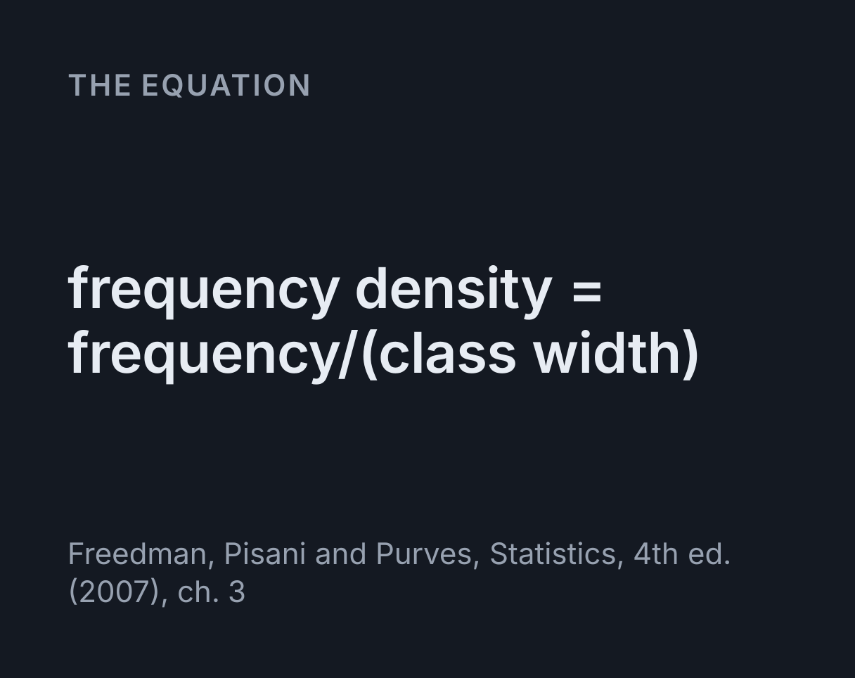
The equation
Freedman, Pisani and Purves, Statistics, 4th ed. (2007), ch. 3
What is frequency density?
Frequency density is the frequency of a class divided by its class width:
frequency density = frequency ÷ class width. It goes on the vertical axis of a
histogram, and that makes the area of each bar equal to the frequency of its class, because
frequency density × class width = frequency. Area, not height, is what a histogram
asks you to compare, which is how it can show classes of different widths fairly.
Its unit is the frequency per unit of whatever was measured. The calculator opens on the journey
times of 80 commuters, so its frequency densities are in commuters per minute: the 11 commuters
who took between 10 and 15 minutes are spread over 5 minutes, which is
11 ÷ 5 = 2.2 commuters per minute. The textbook Statistics by Freedman,
Pisani and Purves calls this vertical axis the density scale.
Using the calculator
Each row of the class table is one class. Type the lower boundary of the first class, then the upper boundary and the frequency of each class in turn. A class starts where the one before it ends, because the bars of a histogram meet with no gaps between them. Add a class or remove the last one with the buttons under the rows, and type what was measured, with its unit, to label the horizontal axis.
The histogram redraws as you type. The number over each bar is its frequency density, the darker bar is the modal class, the dashed line marks the estimated median and the dotted line the estimated mean. Type a pair of values into the last two boxes and the shaded area is the estimate of how many items lie between them. Under the histogram, the table gives each class’s width, frequency density, midpoint, f × x and cumulative frequency, and the working sets out every sum with your numbers in it.
Worked example: 80 commuters’ journey times
The opening table has five classes of unequal width: 0 to 10 minutes with 6 commuters, 10 to 15 with 11, 15 to 20 with 19, 20 to 30 with 20 and 30 to 60 with 24.
- Frequency densities.
6 ÷ 10 = 0.6,11 ÷ 5 = 2.2,19 ÷ 5 = 3.8,20 ÷ 10 = 2and24 ÷ 30 = 0.8. These are the bar heights. - Modal class. The tallest bar is 15 to 20 minutes, at 3.8. The 30 to 60 class holds more commuters, 24, but they are spread over 30 minutes, so its bar is one of the lowest.
- Mean. The midpoints are 5, 12.5, 17.5, 25 and 45, so
Σfx = 6 × 5 + 11 × 12.5 + 19 × 17.5 + 20 × 25 + 24 × 45 = 2080and the estimated mean is2080 ÷ 80 = 26minutes. - Median. Half of 80 is 40. The cumulative frequency is 36 at 20 minutes and 56
at 30, so the median lies in the 20 to 30 class:
20 + (40 − 36) ÷ 20 × 10 = 22minutes. - Frequency between 25 and 40 minutes. The area between the two values is
2 × 5 = 10from the 20 to 30 bar and0.8 × 10 = 8from the 30 to 60 bar, so about10 + 8 = 18commuters took between 25 and 40 minutes.
The mean is 4 minutes above the median because the long last class pulls it upwards, the usual
sign of data skewed to the right. The readouts also give an interquartile range of
35 − 15.79 = 19.21 minutes and an estimated standard deviation of 13.56 minutes.
Why unequal class widths need frequency density
Draw the same table with frequency on the vertical axis and the 30 to 60 bar becomes the tallest.
Being 30 minutes wide as well, it covers more of the chart than the other four bars put together,
and a reader comparing areas would conclude that most commuters take over half an hour, when 24
of 80 do. Dividing by the width removes the distortion: the bar keeps exactly the area it should,
0.8 × 30 = 24, by being low and wide.
Area is also how a histogram is read. The number of items in any range is the area over that range, and the total area is the total frequency, 80 here. It is the same idea as approximating the area under a curve with rectangles in the Riemann sum explorer. Some exam questions scale the axis so that one square of the grid stands for a number of items, which makes area proportional to frequency rather than equal to it, so find what one square is worth first.
Estimating from grouped data
Once data are grouped the individual values are gone, so the mean, median and mode can only be
estimated. The mean counts every item at its class midpoint. The median and the quartiles assume
the items in a class are spread evenly across it, which is linear interpolation:
median = L + (n ÷ 2 − F) ÷ f × w, where L is the lower boundary of the median class,
F the cumulative frequency before it, f its frequency and w its width. The quartiles use n ÷ 4
and 3n ÷ 4 in the same way. The standard deviation is estimated as
√(Σfx² ÷ n − mean²), dividing by n as school courses do for grouped data. When you
have the raw values rather than a table, the
standard deviation calculator gives the exact
mean, median and spread instead.
What this model leaves out
- Where values sit inside a class. Every estimate assumes the items are spread evenly through their class, or sit at its midpoint. Real data rarely are, so the estimated mean can be out by up to half the widest class width.
- Open-ended classes. A class such as “60 or more” has no width, so it has no frequency density and no bar. Choose a sensible upper boundary and say that you did.
- Class limits. Whole numbers grouped as 10 to 19 and 20 to 29 leave gaps between the printed limits. Enter the class boundaries, 9.5, 19.5 and 29.5, so each class is 10 wide and the bars meet.
- Two variables at once. A histogram describes one measured quantity. To see how one quantity changes with another, the linear regression calculator fits a line of best fit, and the error bars and worst-fit line calculator finds the uncertainty in its gradient.
Common mistakes
- Plotting frequency instead of frequency density. With unequal widths the wide classes then look far bigger than they are.
- Taking the class with the highest frequency as the modal class. The modal class has the highest frequency density: it is the tallest bar.
- Reading a frequency off the vertical axis. The height is a density. Multiply it by the width of the bar, or of the part of the bar you need.
- Working out widths from class limits. A class of 10 to 19 whole marks runs from 9.5 to 19.5, so it is 10 wide, not 9.
- Dividing Σfx by the number of classes. Divide by the total frequency, 80 here, not by 5.
- Giving the median class as the median. The 20 to 30 class says where the median is; interpolation gives the estimate, 22 minutes.
Common questions
How do you calculate frequency density?
Divide the frequency of each class by its class width, the upper class boundary minus the lower one. A class from 10 to 15 minutes holding 11 commuters has a frequency density of 11 ÷ 5 = 2.2 commuters per minute. For whole-number data use the class boundaries, not the printed limits: a class of 10 to 19 runs from 9.5 to 19.5 and is 10 wide.
Why does a histogram use frequency density instead of frequency?
So that the area of each bar, frequency density × class width, equals its frequency. With unequal class widths, bars as tall as their frequencies make the wide classes look far bigger than they are. In the calculator’s opening data the 30 to 60 minute class has the most commuters, 24, but it is 6 times as wide as the 5 minute classes, so its bar is only 0.8 high while the 15 to 20 bar reaches 3.8.
How do you find the frequency from a histogram?
Multiply the bar’s frequency density by its width: the area of the bar is the frequency. For part of a class, multiply the bar’s height by the width of the part you need, which assumes the items are spread evenly across the class. Between 25 and 40 minutes in the opening data that is 2 × 5 = 10 from the 20 to 30 bar plus 0.8 × 10 = 8 from the 30 to 60 bar, so about 18 commuters.
How do you estimate the mean from grouped data?
Multiply each class midpoint by its frequency, add the products and divide by the total frequency: mean ≈ Σfx ÷ Σf. For the opening data that is 2080 ÷ 80 = 26 minutes. It is an estimate because every value in a class is counted as if it were at the midpoint, so it can be out by up to half the widest class width.
Is the modal class the class with the highest frequency?
Not necessarily. The modal class is the one with the highest frequency density, the tallest bar on the histogram. When every class has the same width that is always the class with the highest frequency, but with unequal widths it often is not. In the opening data the 15 to 20 minute class has 19 commuters, fewer than the 24 in the 30 to 60 class, but its frequency density of 3.8 is the highest, so it is the modal class.
Should I use n ÷ 2 or (n + 1) ÷ 2 for the median of grouped data?
Use n ÷ 2, which is the usual convention for grouped data and the one this calculator follows. A few textbooks use (n + 1) ÷ 2. For the opening data n ÷ 2 = 40 gives 20 + (40 − 36) ÷ 20 × 10 = 22 minutes and (n + 1) ÷ 2 = 40.5 gives 22.25, so the difference is small, and it shrinks as n grows.