Linear Regression Calculator
Paste two columns of data to get the least-squares line of best fit: slope and intercept with standard errors, 95% intervals, r, r² and residuals.
Calculator
Two columns, x first and then y, one point per line. Paste them from a spreadsheet or type them separated by tabs, commas or spaces. A first line of column names labels the axes.
5 points read. Columns: Current (mA) as x, Voltage (V) as y.
- Least-squares line
- Measured points
- Slope The gradient m, with one standard error. Its unit is the unit of y divided by the unit of x.
- 1.98 ± 0.04
- Intercept Where the line crosses x = 0, c, with one standard error, in the unit of y.
- 0.16 ± 0.14
- r² The fraction of the variation in y that the line accounts for. It cannot tell a straight line from a gentle curve: the residual plot can.
- 0.99857
- n
- 5
Slope
- Value
- 1.98
- Standard error
- 0.0432
- 95% interval
- 1.8425 to 2.1175
- Reported at 95%
- 1.98 ± 0.14
Intercept
- Value
- 0.16
- Standard error
- 0.1433
- 95% interval
- −0.29596 to 0.61596
- Reported at 95%
- 0.2 ± 0.5
- Interval includes zero
- Yes
Fit
- Equation
- y = 1.98x + 0.16
- r
- 0.99929
- r²
- 0.99857
- Residual SD, s
- 0.13663
- Degrees of freedom
- 3
- t critical (95%)
- 3.182
- Zero
- Residuals
Residuals for each point
| Point | Current (mA) | Voltage (V) | Line | Residual |
|---|---|---|---|---|
| 1 | 1 | 2.2 | 2.14 | 0.06 |
| 2 | 2 | 4.1 | 4.12 | −0.02 |
| 3 | 3 | 6.1 | 6.1 | 0 |
| 4 | 4 | 7.9 | 8.08 | −0.18 |
| 5 | 5 | 10.2 | 10.06 | 0.14 |
Working
- n = 5
- mean x = 15 / 5 = 3
- mean y = 30.5 / 5 = 6.1
- Sxx = Σ(x - mean x)^2 = 10
- Sxy = Σ(x - mean x)(y - mean y) = 19.8
- Syy = Σ(y - mean y)^2 = 39.26
- slope m = Sxy / Sxx = 19.8 / 10 = 1.98
- intercept c = mean y - m × mean x = 6.1 - 1.98 × 3 = 0.16
- residual sum of squares SSE = Σ(y - mx - c)^2 = 0.056
- residual SD s = sqrt(SSE / (n - 2)) = sqrt(0.056 / 3) = 0.13663
- SE of slope = s / sqrt(Sxx) = 0.13663 / sqrt(10) = 0.043205
- SE of intercept = s × sqrt(1/n + mean x^2 / Sxx) = 0.13663 × sqrt(1/5 + 3^2 / 10) = 0.14329
- r = Sxy / sqrt(Sxx × Syy) = 19.8 / sqrt(10 × 39.26) = 0.99929
- r^2 = 1 - SSE / Syy = 1 - 0.056 / 39.26 = 0.99857
- t (95%, 3 degrees of freedom) = 3.182
- slope 95% half-width = 3.182 × 0.043205 = 0.13748
- intercept 95% half-width = 3.182 × 0.14329 = 0.45596
- m = 1.98 ± 0.04, c = 0.16 ± 0.14 (± one standard error)
Each sum is taken about the means, which gives the same slope as the textbook formula without the rounding error that formula suffers when x is large.
Citing this tool
Last updated . Add the date you accessed it as well, which a citation of a page that can change asks for. If a specific result matters, cite the permalink from the tool’s share row instead of this page: it reproduces the exact parameters.
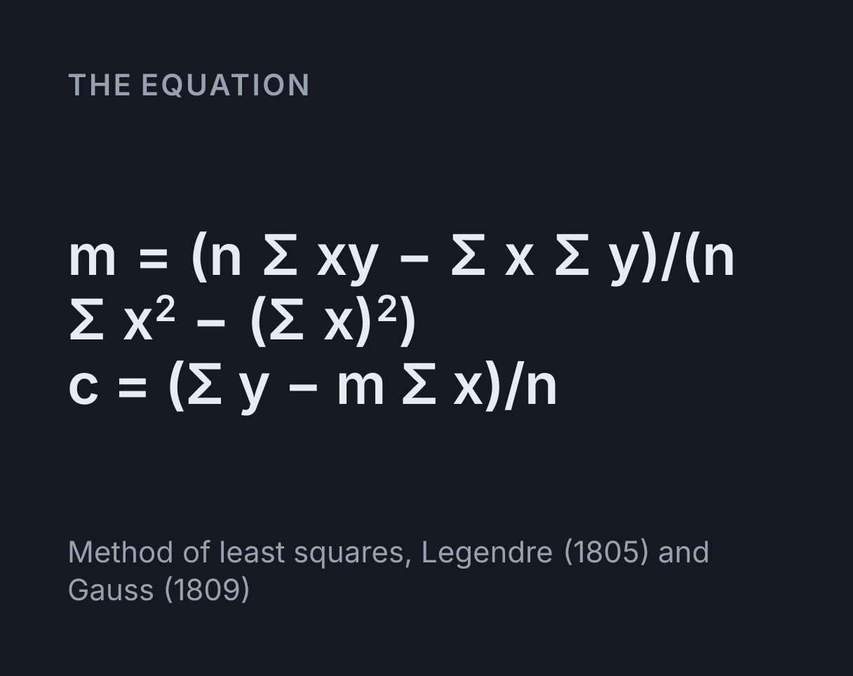
The equation
Method of least squares, Legendre (1805) and Gauss (1809)
The least-squares line of best fit
Linear regression finds the straight line y = mx + c that makes the sum of the
squared vertical distances from the points to the line as small as possible, which gives
m = (nΣxy − ΣxΣy) / (nΣx² − (Σx)²) and c = (Σy − mΣx) / n. Those
vertical distances are the residuals, each measured y minus the line’s value
at the same x.
The slope is also written m = Sxy / Sxx, where Sxx is the sum of the
squared deviations of x from its mean and Sxy is the sum of the products of the
deviations of x and y. That is the form the calculator uses. It is the same number, but it
takes the means away before multiplying, where the textbook sums subtract two large, nearly
equal totals at the end. With the currents in the example below shifted by a billion, the
textbook sums in double precision give an infinite slope; the deviations still give 1.98.
How to use it
Paste two columns from a spreadsheet, x first and then y, or type one point per line with the two numbers separated by a tab, a comma or spaces. A first line of column names labels the axes and the table. Any line that does not hold exactly two numbers is skipped and listed under the box, so a typing error cannot quietly shrink the data.
Typical uses: a resistance from voltage against current, as in the example below; a spring constant from force against extension; and a calibration line of absorbance against concentration, whose slope is εl in the Beer-Lambert law.
The slope and intercept are shown with one standard error, rounded to the decimal place that error allows, and the panels below give the 95% interval of each, r, r², the residual standard deviation and the degrees of freedom. The residual plot and the table under it show how far each point sits from the line. The working lists every sum with your numbers, so a hand calculation can be checked line by line, and the CSV download holds the points, the line’s value at each and the residuals at full precision.
Worked example: a resistance from five readings
A resistor’s voltage is read at five currents, which is the data the calculator opens with: 1, 2, 3, 4 and 5 mA give 2.2, 4.1, 6.1, 7.9 and 10.2 V.
- Means:
mean x = 15 / 5 = 3mA andmean y = 30.5 / 5 = 6.1V. - Sums of deviations:
Sxx = 10,Sxy = 19.8andSyy = 39.26. - Slope:
m = 19.8 / 10 = 1.98V/mA, which is a resistance of 1.98 kΩ. - Intercept:
c = 6.1 − 1.98 × 3 = 0.16V. -
Residuals:
0.06, −0.02, 0, −0.18, 0.14V, whose squares add up toSSE = 0.056. -
Residual standard deviation:
s = √(0.056 / 3) = 0.1366V, dividing by three rather than five because the line has used two of the five degrees of freedom. -
Standard errors:
0.1366 / √10 = 0.0432V/mA for the slope and0.1366 × √(1/5 + 3² / 10) = 0.1433V for the intercept. - Correlation:
r = 19.8 / √(10 × 39.26) = 0.99929, sor² = 0.99857.
The resistance is 1.98 ± 0.04 kΩ quoting one standard error, or 1.98 ± 0.14 kΩ at 95% confidence, where the multiplier is t = 3.182 for three degrees of freedom. The intercept is 0.16 ± 0.14 V, and its 95% interval, −0.30 to 0.62 V, includes zero, so the data are consistent with Ohm’s law and a line through the origin. Forcing the line there gives 2.024 ± 0.019 kΩ.
The uncertainty in the slope and intercept
The standard error of the slope is s / √Sxx and that of the intercept is
s × √(1/n + (mean x)² / Sxx), where s = √(SSE / (n − 2)) is the
residual standard deviation, the typical scatter of the points about the line in the units of
y. The divisor is n − 2 because the line spends one degree of freedom on each of
its two parameters, for the same reason a
sample standard deviation divides by
n − 1.
A standard error is one standard deviation of the estimate. For a 95 percent interval,
multiply it by the t value for n − 2 degrees of freedom: 4.303 for four points,
3.182 for five, 2.306 for ten and still 2.042 at 32. Using 1.96 with four points makes the
interval less than half as wide as it should be. Conventions differ between subjects and lab
manuals, so say which of the two you quote, and round the value to the decimal place of its
uncertainty, as the readouts above do.
School physics courses often find the uncertainty in the gradient graphically instead: draw the steepest and shallowest lines that still pass through every error bar, and take the uncertainty from how far their gradients differ from the best-fit one. That method rests on the error bars rather than on the scatter of the points, so it gives a different number from the standard error, and a report should say which one it quotes.
These are the same quantities Excel’s LINEST function returns as m, b, se1, seb, r2 and sey, so a spreadsheet can check them. The arithmetic here is also tested against the certified answers NIST publishes for exactly this purpose, its Statistical Reference Datasets for linear regression, including the two for a line through the origin.
Reading r, r² and the residuals
r measures how closely the points follow a straight line, from −1 to 1, and r² is the fraction of the variation in y that the line accounts for. Neither says whether a straight line is the right shape. Anscombe’s quartet, published in 1973, is four sets of eleven points with the same slope, intercept and r² to two decimal places: one is ordinary scatter about a line, one is a smooth curve, one is an exact line with a single outlier, and one is a vertical cluster whose slope is set entirely by one distant point.
The residual plot under the results is the check. Residuals scattered evenly about zero support a straight line. A bow, with the residuals on one side of zero at both ends and on the other in the middle, means the relationship curves. A funnel that widens along x means the scatter is not constant. A single residual far from the rest is a reading to recheck, which is a prompt to investigate, not a licence to delete it.
When to force the line through the origin
Tick Force the line through the origin and the fit becomes y = mx, with
m = Σxy / Σx² and s = √(SSE / (n − 1)), since only one parameter is
fitted. Do it when theory requires y to be zero at x = 0 and the free line agrees. While the
box is ticked the calculator says whether the free line’s intercept has a 95% interval that
includes zero. If it does not, the data carry an offset, such as an unzeroed balance, an
unsubtracted blank or a meter that does not read zero, and forcing the line through the
origin hides it by tilting the slope.
For a line through the origin, R² is measured about zero rather than about the mean of y, which is how NIST’s reference datasets and Excel’s LINEST define it for this model. It usually runs higher than the free line’s r² for the same data, 0.99965 against 0.99857 in the example, and the two cannot be compared.
What this does not cover
It weights every point equally, which assumes each y carries the same uncertainty and each x is exact. Points with their own error bars need weighted least squares, with weights proportional to 1/σ², as the NIST/SEMATECH e-Handbook of Statistical Methods sets out, and uncertainty in x as well needs an errors-in-variables fit such as Deming regression. It fits straight lines only, so a curve needs a nonlinear fit. It gives 95 percent intervals rather than p-values: a slope whose interval excludes zero is significant at the 5 percent level. It does not draw confidence or prediction bands, and it does not read an unknown back off a calibration line, which needs an uncertainty formula of its own.
Common mistakes
- Treating r² as the uncertainty. r² describes the scatter, not how well the slope is known. The example’s r² of 0.9986 still leaves its slope uncertain by 7 percent at 95 percent confidence.
- Using 1.96 for a small data set. With five points the 95 percent multiplier is 3.182, and with three it is 12.706.
- Forcing the line through the origin because the theory says so. Fit the free line first and look at its intercept. An offset that the theory does not allow is a finding about the apparatus, and forcing the line through zero hides it.
- Straightening a curve and trusting the fit. Taking logarithms or reciprocals to make a curve straight also reshapes its scatter, so weighting every point equally is no longer right. The Lineweaver-Burk plot in the Enzyme Kinetics Simulator is the standard example.
- Reading the line beyond the data. The fit is only tested where there are points. Outside that range nothing shows that the relationship stays straight.
- Pasting the columns the wrong way round. The first column is x. Least squares treats all the scatter as belonging to y, so swapping the columns fits a different line rather than the same line turned round.
To carry the slope’s uncertainty into a quantity calculated from it, such as a spring constant or an acceleration, use the Error Propagation Calculator, and to compare the result with an accepted value, the Percent Error Calculator.
Common questions
How do I find the uncertainty in the slope of a line of best fit?
Use the standard error of the slope, s divided by the square root of Sxx, where s is the residual standard deviation, the scatter of the points about the line, and Sxx is the sum of the squared deviations of x from its mean. For a 95% interval multiply it by the t value for n − 2 degrees of freedom, which for five points is 3.182 rather than 1.96. This calculator shows both, with the slope rounded to the place its uncertainty allows. School physics courses often use the steepest or shallowest line through the error bars instead, which rests on the error bars rather than the scatter and gives a different number.
What is the difference between r and r²?
r is the correlation coefficient, which runs from −1 to 1 and takes the sign of the slope, and r² is its square, the fraction of the variation in y that the line accounts for. An r of 0.9 sounds strong, but its r² of 0.81 leaves nearly a fifth of the variation in y unexplained. For a line forced through the origin R² is measured about zero instead of about the mean, so it usually runs higher and cannot be compared with the free line’s.
Does a high r² mean the data are linear?
No. r² measures how much of the scatter a straight line removes, not whether a straight line is the right shape. Anscombe’s quartet (1973) is four sets of eleven points that share a slope of 0.500, an intercept of 3.00 and an r² of 0.67, and one of them is a smooth curve while another is a straight line thrown off by a single outlier. Check the residual plot: points scattered evenly about zero support a line, and a curve or a funnel says it is the wrong model.
Should I force the line of best fit through the origin?
Only when theory says y must be zero when x is zero and the data agree. Fit the free line first. If the intercept’s 95% interval includes zero, a line through the origin is consistent with the data and usually gives a more precise slope. If the interval excludes zero there is an offset, such as an unzeroed balance or an unsubtracted blank, and forcing the line through zero hides it and biases the slope.
Does it matter which variable goes on the x axis?
Yes. Least squares minimises the vertical distances from the points to the line, so it treats all the scatter as belonging to y. Fitting y against x and x against y gives two different lines unless every point lies on one, and their slopes multiply to r², not to 1. Put the quantity you set or measured most precisely on the x axis, which is usually the independent variable.