Enzyme Kinetics Simulator

One equation, and where the inhibitors go into it

An inhibitor can bind the free enzyme, the enzyme-substrate complex, or both. Each route multiplies one term of the Michaelis-Menten denominator, and that is the whole of it:

• α = 1 + [I]/Ki, for an inhibitor binding free enzyme. It scales the Km term.
• α′ = 1 + [I]/Ki′, for an inhibitor binding the ES complex. It scales the [S] term.

So v = Vmax[S] / (αKm + α′[S]). Divide through by α′ and it is Michaelis-Menten again, with apparent constants Km_app = αKm/α′ and Vmax_app = Vmax/α′. Every case below is those two expressions with different numbers in them, which is worth knowing because it means there is nothing extra to memorise.

Telling the three modes apart, by which intercept stays fixed

On the direct curve the three inhibitors look confusingly similar: a shifted curve is just a shifted curve, and two of the three lower the plateau. The Lineweaver-Burk plot separates them instantly, because the lines it draws pin down Km and Vmax independently: the vertical intercept is 1/Vmax_app and the horizontal intercept is −1/Km_app.

• Competitive. The inhibitor competes for the active site, so it only affects free enzyme: α > 1, α′ = 1. Apparent Km rises by α; Vmax does not move at all. The lines share the y intercept.
• Non-competitive, pure. The inhibitor binds elsewhere and binds free enzyme and the ES complex equally well: α = α′ > 1. Apparent Vmax falls by α; Km does not move. The lines share the x intercept.
• Uncompetitive. The inhibitor binds only the ES complex, so it needs the substrate to be there first: α = 1, α′ > 1. Apparent Km and apparent Vmax both fall by α′, so the slope Km/Vmax is unchanged and the lines are parallel.

There is a fourth case, mixed inhibition, where α and α′ are both above 1 but unequal. Both constants then move and no intercept is preserved, which is chemically common and diagnostically unhelpful. The simulator sticks to the three canonical patterns, because recognising those is the skill being practised.

The best test of a competitive inhibitor is not a plot at all. Drag the substrate slider up with competitive selected and watch the percent of the true Vmax climb back towards 100. A competitive inhibitor and the substrate are fighting over the same site, so enough substrate wins. Do the same with non-competitive selected and it stalls at 1/α, no matter how much substrate you add, because the ceiling itself has moved down. That single experiment distinguishes the two mechanisms without drawing anything.

What Km actually measures

Km is the substrate concentration at which the enzyme runs at half its maximum rate. That is the definition, and it is a definition about rate, not about binding.

Calling Km an affinity is a useful approximation rather than a synonym. For the simple mechanism E + S ⇌ ES → E + P, Km = (k₋₁ + k₂)/k₁, whereas the dissociation constant of the ES complex is Kd = k₋₁/k₁. The two coincide only when k₂ ≪ k₋₁, that is, when catalysis is much slower than the substrate falling back off. Plenty of enzymes are not like that. For a fast one, Km can be far larger than Kd, and calling it the affinity then understates the binding badly.

What is reliably true is that Km is a property of the enzyme and substrate pair rather than of how much enzyme is present. Raise Vmax in the simulator, which is what adding enzyme does, and Km does not move. That asymmetry is the most useful thing about the pair of constants.

Why the curve saturates

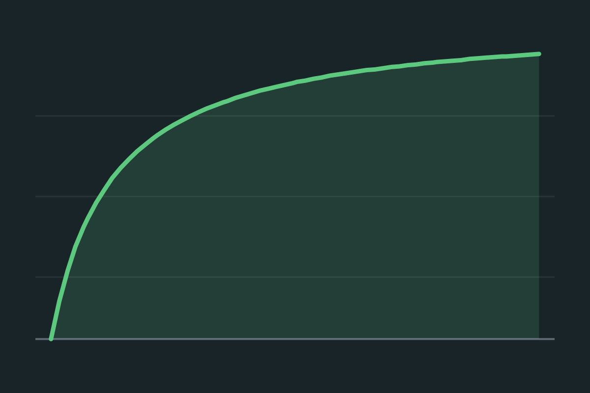
There is a fixed amount of enzyme. At low substrate almost all of it is sitting empty, so the rate is limited by how often an enzyme meets a substrate molecule: double the substrate and you roughly double the rate. That is first order kinetics, and it is the steep part of the curve near the origin.

At high substrate essentially every active site is already occupied. Adding more substrate changes nothing, because the limit is now how fast each enzyme can process what it is already holding. The rate becomes independent of substrate concentration, which is zero order kinetics, and the ceiling is Vmax. Km marks the crossover between the two regimes, and it takes nine times Km to reach 90 percent of Vmax, which is why saturation curves flatten so lazily.

This is also why pharmacology cares. A drug cleared by an enzyme working well below Km clears at a rate proportional to its concentration, so it has a half life. A drug that saturates the enzyme clears at a fixed amount per hour instead, so the dose response stops being linear. Ethanol is the standard example.

Why Lineweaver-Burk survives despite being statistically poor

Taking reciprocals distorts the error structure badly. The high-substrate measurements, which are the largest velocities and therefore the most precisely measured, all get squeezed into a small cluster near 1/[S] = 0. The low-substrate measurements, which are the smallest velocities and carry the largest relative error, get spread out across the rest of the axis. A straight line fitted by eye or by unweighted least squares is then dominated by the least reliable data, and the resulting Km and Vmax are biased.

Nobody determines kinetic constants that way now. The correct method is a nonlinear least squares fit straight to the hyperbola, using the measurements as they were made, which is a few lines of code in any statistics package. The Eadie-Hofstee and Hanes-Woolf plots are better-behaved linearisations and are also obsolete for fitting.

Lineweaver-Burk survives anyway, and it deserves to, because no other plot identifies mechanism at a glance. Two straight lines that meet on the vertical axis, meet on the horizontal axis, or never meet at all is about as clear as a diagnostic gets. Use it to see what kind of inhibition you have; use a nonlinear fit to say what the numbers are.

What this model leaves out

The Michaelis-Menten assumptions, all of which the simulator inherits. One substrate and one product. A steady state, so the concentration of the ES complex is treated as constant, which requires substrate in large excess over enzyme. No product yet accumulated, so no product inhibition, and no reverse reaction, so the measured velocity is the initial velocity only. Real assays drift away from every one of these as they run, which is why initial rates are what get measured.

The important omission is bigger than any of those. This model cannot describe an allosteric or cooperative enzyme at all. An enzyme with multiple interacting subunits does not give a hyperbola; it gives a sigmoid, with a shallow foot, a steep middle and a plateau, because substrate binding at one site changes the affinity of the others. Phosphofructokinase is the textbook case: it sits at the committed step of glycolysis and its sigmoid response, tuned by ATP and AMP and citrate, is what makes it a control point rather than a mere catalyst. Fitting a hyperbola to a sigmoid does not give a slightly wrong Km. It gives a number that means nothing, and the Hill equation is the right starting point instead.

Also absent: irreversible inhibitors, which knock enzyme out permanently rather than binding reversibly, so aspirin on cyclooxygenase is nothing like anything modelled here. Temperature and pH, both of which move Vmax and Km together. And multi-substrate mechanisms, where the ordering of binding matters and there is more than one Km to speak of.

Common mistakes

• Confusing uncompetitive with non-competitive. The most common error in this whole topic, and the two words are not synonyms. Uncompetitive means the inhibitor binds only the ES complex, so Km and Vmax fall together and the reciprocal lines are parallel. Non-competitive, in its pure textbook sense, means it binds free enzyme and ES equally, so Vmax falls and Km does not move. Look at what happened to Km: that is what separates them, since both lower Vmax by the same factor.
• Reading Km as a binding constant. It equals the dissociation constant only when catalysis is slow relative to dissociation. Otherwise it is larger, sometimes much larger.
• Expecting the curve to reach Vmax. It never does. Saturation is asymptotic, which is exactly why the useful constant is defined at half of it.
• Thinking a competitive inhibitor lowers Vmax. It cannot. Given enough substrate the enzyme reaches its full rate. What the inhibitor costs you is the substrate needed to get there.
• Reporting Vmax/Km as the specificity constant. The specificity constant is kcat/Km, and kcat = Vmax/[E]total, so it needs the enzyme concentration. Vmax/Km is proportional to it for a fixed amount of enzyme and is not the same number.
• Fitting a straight line to sigmoid data. If a Lineweaver-Burk plot of real measurements curves, the enzyme is very likely cooperative, and the answer is a different model rather than a better line.
• Comparing Km values measured under different conditions. Both constants depend on temperature, pH and ionic strength, so a Km from one paper and a Km from another are not necessarily comparable.