Mark-Recapture Population Calculator
Mark-recapture calculator: population size by the Lincoln-Petersen index and Chapman’s estimator, with standard error, a 95% interval and full working.
Calculator
- 12 marked
- 28 unmarked
12 of the 40 caught are marked, 30% of the sample. If the 30 marked animals are 30% of the whole population, N = 30 × 40 ÷ 12 = 100.
- Lincoln-Petersen N N = M × C ÷ R: the population in which the marked share, M ÷ N, equals the marked share of the second sample, R ÷ C.
- 100
- Chapman N N = (M + 1)(C + 1) ÷ (R + 1) − 1, Chapman’s 1951 correction. It removes most of the small-sample bias of the Lincoln-Petersen figure and stays finite when R = 0.
- 96.77
- 95% interval Chapman’s N ± 1.96 standard errors, a normal approximation. It is rough when R is small, because the real spread of estimates is lopsided.
- 64.5 to 129.0
- Standard error The square root of Seber’s 1970 variance for Chapman’s N: (M + 1)(C + 1)(M − R)(C − R) ÷ [(R + 1)²(R + 2)].
- 16.45
- Marked share, R ÷ C R ÷ C, the fraction of the second sample that carries a mark. The method assumes the whole population has the same fraction marked.
- 0.3
- Different animals caught M + C − R, the animals caught at least once. The population cannot be smaller than this.
- 58
Working
- M = 30 marked first, C = 40 caught second, R = 12 of them marked.
- marked share of the second sample, R / C = 12 / 40 = 0.3
- Assume the same share of the whole population is marked: M / N = R / C.
- Lincoln-Petersen N = 30 x 40 / 12 = 100
- Chapman N = (30 + 1) x (40 + 1) / (12 + 1) - 1 = 96.769
- variance = 31 x 41 x 18 x 28 / (13^2 x 14) = 270.75
- standard error = sqrt(270.75) = 16.454
- lower 95% limit = 96.769 - 1.96 x 16.454 = 64.519
- upper 95% limit = 96.769 + 1.96 x 16.454 = 129.02
- different animals caught, M + C - R = 30 + 40 - 12 = 58
M × C ÷ R is the textbook answer. Chapman’s N is the better single figure to report, with its interval, because it removes most of the bias small samples give the Lincoln-Petersen figure.
Citing this tool
Last updated . Add the date you accessed it as well, which a citation of a page that can change asks for. If a specific result matters, cite the permalink from the tool’s share row instead of this page: it reproduces the exact parameters.
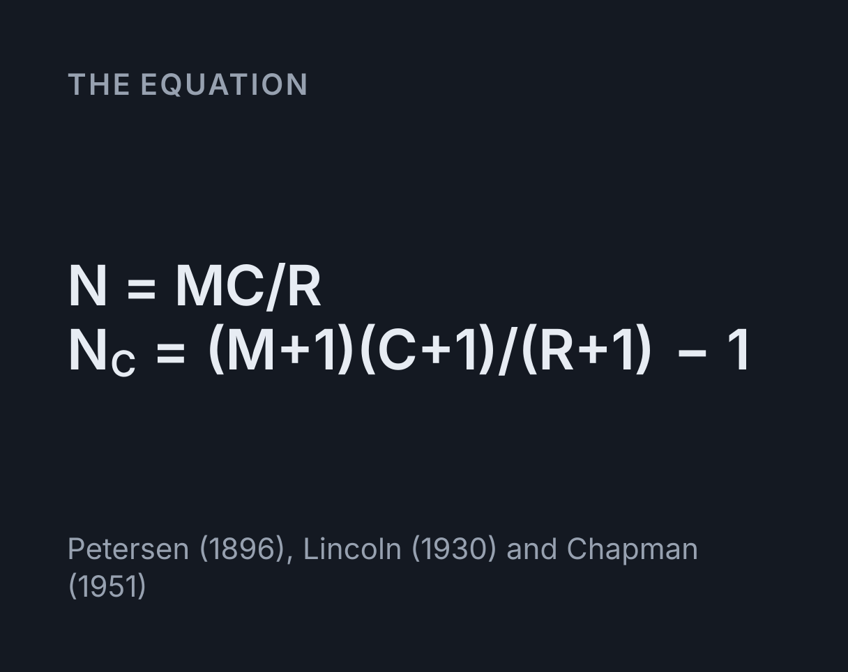
The equation
Petersen (1896), Lincoln (1930) and Chapman (1951)
How mark-recapture estimates population size
Mark-recapture estimates how many animals live in an area without counting every one. Catch
a first sample of M animals, mark each one and release it. Later, catch a second sample of C
animals and count the R of them that carry a mark. If the marked animals have mixed back in
at random, the marked share of the second sample estimates the marked share of the whole
population, R ÷ C = M ÷ N, so the population size is
N = M × C ÷ R.
That is the Lincoln-Petersen estimate, also called the Lincoln index. It is named after the Danish fisheries biologist C. G. J. Petersen, who tagged plaice in the 1890s, and the American ornithologist Frederick Lincoln, who estimated waterfowl numbers from bird-banding returns in 1930. British specifications call the fieldwork mark-release-recapture, and some books write n₁, n₂ and m₂ for M, C and R. This calculator gives the Lincoln-Petersen figure beside Chapman’s less biased version, the standard error and an approximate 95 percent interval, and draws the second sample so that the ratio behind the answer can be seen.
Using the calculator
Enter the three counts. M is every animal marked and released on the first visit. C is everything caught on the second visit, marked or not, and R is how many of those carry a mark. The slider for R runs only up to the smaller of M and C, because the recaptures belong to both groups.
The diagram draws the second sample, a filled dot for each marked animal and a hollow ring for each unmarked one, with the marked dots spread evenly through the grid, as the method assumes marked animals are spread through the population. Above 400 animals each dot stands for 1 percent of the sample. The readouts give both estimates, the standard error and interval of Chapman’s estimate, the marked share R ÷ C, and M + C − R, the number of different animals caught, which is the least the population can be. A note appears under the readouts when the counts are too few to trust, and the working sets out every step with your numbers.
For the rest of an ecology write-up, the Simpson’s diversity index calculator turns quadrat and sweep-net counts into a diversity index, and for plant physiology the water potential calculator covers osmosis in plant cells.
Worked example: 30 marked, 40 caught, 12 recaptured
These are the values loaded above. A student marks 30 woodlice with a dot of non-toxic paint, releases them where they were found and comes back the next day to catch 40, of which 12 are marked.
- Marked share of the second sample:
12 ÷ 40 = 0.3. - Lincoln-Petersen:
N = 30 × 40 ÷ 12 = 100, the same as30 ÷ 0.3. - Chapman:
N = 31 × 41 ÷ 13 − 1 = 96.77. -
Variance:
31 × 41 × 18 × 28 ÷ (13² × 14) = 640,584 ÷ 2,366 = 270.75. - Standard error:
√270.75 = 16.454. -
95 percent interval:
96.77 ± 1.96 × 16.454 = 96.77 ± 32.25, which is 64.5 to 129.0. -
Different animals caught:
30 + 40 − 12 = 58, so there are at least 58 woodlice.
So the best single figure is about 97 woodlice, and the counts are consistent with anything from about 65 to 129. Chapman’s figure is 3.2 percent below the Lincoln-Petersen 100, and its standard error is 17 percent of the estimate.
Chapman’s estimator and the 95 percent interval
The Lincoln-Petersen formula overestimates on average, and with small samples it can fail
outright: if no marked animal turns up in the second sample, R = 0 and it divides by zero.
Chapman (1951) adjusted it to N = (M + 1)(C + 1) ÷ (R + 1) − 1. This is exactly
unbiased whenever M + C is at least the true population size, stays finite at R = 0, and
comes very close to the Lincoln-Petersen figure once R is large, so it is the better single
number to report.
The variance usually quoted with it is Seber’s (1970):
Var = (M + 1)(C + 1)(M − R)(C − R) ÷ [(R + 1)²(R + 2)]. Its square root is the
standard error, and adding and subtracting 1.96 standard errors gives an approximate 95
percent interval. This is a normal approximation. When R is small the real spread of possible
estimates is lopsided, with a long tail towards large populations, so the symmetric interval
is rough, and its lower end can even fall below M + C − R, the number of animals you know
exist. The calculator says when that happens. For what a standard error and a confidence
interval mean in general, the
standard deviation calculator works them
out for a set of repeated measurements.
How many animals to mark
Precision depends mostly on the number of recaptures. From the variance above, the standard
error as a share of the estimate is about √[(1 − R ÷ M)(1 − R ÷ C) ÷ R], which
is close to 1 ÷ √R when the recaptures are a small part of both samples. So the
error shrinks only with the square root of R: halving it takes about four times as many
recaptures, and since the number expected is M × C ÷ N, that means doubling both
samples.
In a population of about 1,000, marking 100 and catching 100 should find about 10 marked animals, and the standard error of Chapman’s estimate is then 238.6. Marking and catching 200 each should find about 40, and the standard error falls to 121.0, close to half. A widely used rule of thumb is to plan for at least 7 recaptures; with fewer, the estimate is too uncertain to be much use.
What this model leaves out
- Births, deaths and movement. The method assumes a closed population, with nothing joining or leaving between the samples. Births and immigrants add unmarked animals and push the estimate up. Leave long enough for marked animals to mix back in, but no longer. Over seasons and years numbers rise and fall, as the predator-prey simulator shows for a pair of species.
- Lost or harmful marks. A mark that wears off, or one that makes an animal easier for predators to spot, leaves too few marked animals in the second sample, so the estimate comes out too high.
- Trap-happy and trap-shy animals. If being caught once makes an animal more likely to be caught again, perhaps because the trap was baited, R is too high and N too low. If it makes the animal warier, the error goes the other way.
- Unequal catchability. Some individuals are simply easier to catch, because of their size, sex or behaviour. They turn up in both samples more than their numbers warrant, which raises R and biases the estimate low.
- More than two samples. Repeated sampling, as in the Schnabel method, and models for open populations such as Jolly-Seber use more information than two counts hold.
- Exact small-sample intervals. The normal approximation is the simple textbook interval. Methods built on the binomial or Poisson distribution of R give lopsided intervals that suit a small R better.
Common mistakes
- Swapping C and R.
30 × 12 ÷ 40 = 9, fewer than the 30 animals already marked, which cannot be right. The estimate can never be smaller than M or C. - Leaving the marked animals out of C. C is the whole second catch. Using
only the 28 unmarked animals gives
30 × 28 ÷ 12 = 70instead of 100. - Sampling too soon, or in the same spot. Marked animals released at one place stay near it for a while, so a second sample taken there finds too many of them and the estimate comes out low.
- Reporting too many figures. With 12 recaptures the 95 percent interval runs about 33 percent either side of the estimate, so 96.77 is better reported as about 97, between 65 and 129.
- Reading R = 0 as an infinite population. It means the samples were too small to find a marked animal. Mark and catch more, rather than quoting the formula’s division by zero.
Common questions
How do you calculate population size with mark-recapture?
Multiply the number marked in the first sample, M, by the number caught in the second, C, and divide by the number of marked animals in the second sample, R: N = M × C ÷ R. This is the Lincoln-Petersen estimate, or Lincoln index. With 30 marked, 40 caught and 12 recaptured, N = 30 × 40 ÷ 12 = 100. It works because the marked share of the second sample, 12 in 40 or 30 percent, is taken to be the marked share of the whole population.
What is the Chapman estimator?
A version of the Lincoln-Petersen estimate published by Douglas Chapman in 1951: N = (M + 1)(C + 1) ÷ (R + 1) − 1. The plain formula overestimates on average in small samples and has no answer when R = 0. Chapman’s is exactly unbiased whenever M + C is at least the true population size, and it stays finite at R = 0. With 30 marked, 40 caught and 12 recaptured it gives 31 × 41 ÷ 13 − 1 = 96.77, against 100 from the plain formula.
How do you work out a 95% confidence interval for a mark-recapture estimate?
Find the variance of Chapman’s estimate, (M + 1)(C + 1)(M − R)(C − R) ÷ [(R + 1)²(R + 2)], as given by Seber (1970), take its square root for the standard error, and add and subtract 1.96 standard errors. For 30 marked, 40 caught and 12 recaptured the variance is 270.75, the standard error 16.454 and the interval 96.77 ± 32.25, or 64.5 to 129.0. It is a normal approximation, so treat it as rough when there are few recaptures.
What are the assumptions of the mark-recapture method?
That the population is closed between the samples, with no births, deaths, immigration or emigration; that marks are not lost and do not change how an animal behaves or survives; that marked animals have time to mix back in; and that every animal, marked or not, is equally likely to be caught in the second sample. Lost marks and trap-shy animals push the estimate too high, and trap-happy animals push it too low.
What if no marked animals are recaptured?
Then R = 0 and the Lincoln-Petersen formula divides by zero, so it gives no estimate. Chapman’s formula still gives (M + 1)(C + 1) − 1, which is 1,270 for 30 marked and 40 caught, but its interval is so wide that it shows only that the population is large compared with the samples. A widely used rule of thumb is to aim for at least 7 recaptures, by marking and catching more animals.
Why is it called the Lincoln-Petersen index?
It is named after two biologists who used it. The Danish fisheries scientist C. G. J. Petersen published his work with tagged plaice in 1896, and the American ornithologist Frederick Lincoln estimated waterfowl numbers from bird-banding returns in 1930. The formula is the same in both, N = M × C ÷ R, and British textbooks often call it the Lincoln index.