Oscilloscope Simulator
A two-channel oscilloscope simulator. Set volts/div, time/div, coupling and trigger, read period, peak-to-peak and RMS, and draw Lissajous figures.
Simulator
Drag up or down on the screen to set the trigger level, or use the up and down arrow keys; left and right step the time base. Space plays and pauses.
Oscilloscope screen, 10 by 8 divisions, at 0.2 ms/div. Channel 1: a sine wave, 4 divisions from lowest to highest, one cycle every 5 divisions, with 0 V at 0 divisions from the centre line. Channel 2: a sine wave, 2 divisions from lowest to highest, one cycle every 5 divisions, with 0 V at 0 divisions from the centre line. The trace is locked: each sweep starts where channel 1 crosses 0 V going up.
- Channel 1 peak-to-peak Read off the screen: the trace spans 4 divisions from its lowest point to its highest, and 4 × 1 V/div = 4 V.
- 4 V
- Channel 1 period One cycle spans 5 divisions, and 5 × 0.2 ms/div = 1 ms.
- 1 ms
- Channel 1 frequency f = 1/T = 1/1 ms = 1000 Hz.
- 1000 Hz
- Channel 1 RMS For a sine wave the RMS value is the peak over √2: 2/√2 = 1.414 V.
- 1.414 V
- Trigger Each sweep starts where channel 1 rises through 0 V, 0° into its cycle, so every sweep draws the same trace.
- locked
- Channel 2 peak-to-peak Read off the screen: the trace spans 2 divisions from its lowest point to its highest, and 2 × 1 V/div = 2 V.
- 2 V
- Channel 2 period One cycle spans 5 divisions, and 5 × 0.2 ms/div = 1 ms.
- 1 ms
- Channel 2 frequency f = 1/T = 1/1 ms = 1000 Hz.
- 1000 Hz
- Channel 2 RMS For a sine wave the RMS value is the peak over √2: 1/√2 = 0.7071 V.
- 0.7071 V
- Phase of channel 2 Channel 2 rises through its midline 1.25 divisions after channel 1, out of a 5-division period, so it lags: 360° × 1.25/5 = 90°.
- −90 °
- Channel 1, the trigger source
- Trigger level
Citing this tool
Last updated . Add the date you accessed it as well, which a citation of a page that can change asks for. If a specific result matters, cite the permalink from the tool’s share row instead of this page: it reproduces the exact parameters.
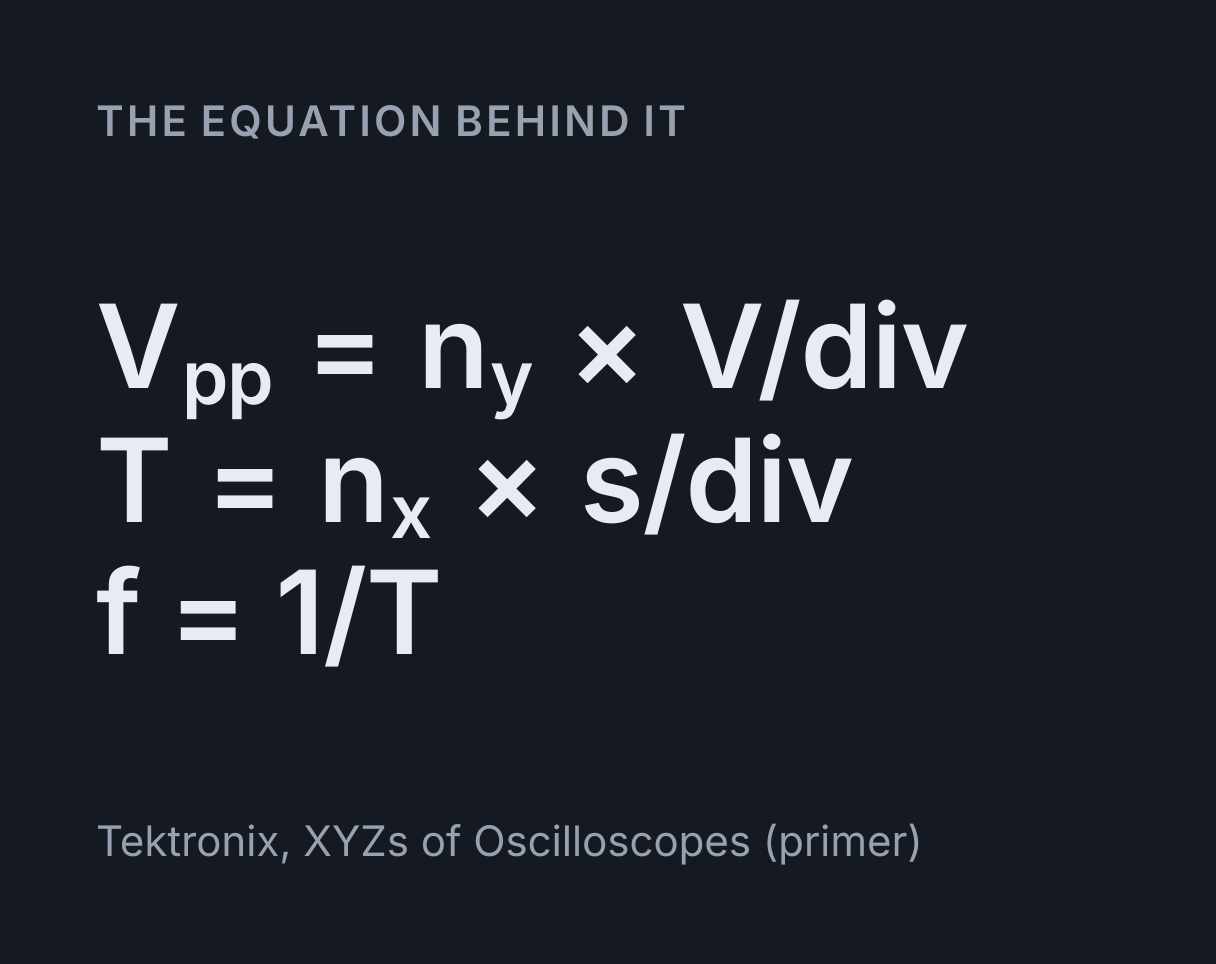
The equation
Tektronix, XYZs of Oscilloscopes (primer)
What is an oscilloscope simulator?
An oscilloscope draws a voltage against time on a grid of squares called divisions, and an
oscilloscope simulator does the same on screen, with signal generators standing in for the
circuit. Every reading comes from counting divisions and multiplying by a knob setting:
V = divisions × volts/div up the screen, T = divisions × time/div
across it, and the frequency is f = 1/T. This one has two channels on a graticule
10 divisions across and 8 up, the classic layout, with a sine, square or triangle generator on
each.
A multimeter gives one number for a steady voltage, which is all the series and parallel circuit simulator needs. A scope shows how a voltage changes, and the simulator models the parts that decide whether you can read it at all: each channel’s vertical scale, position and coupling, the time base, and the trigger that holds the trace still. XY mode switches the time base off and plots one channel against the other, which draws Lissajous figures.
How to use an oscilloscope, step by step
The same routine works on a bench scope and here.
- Find the zero line. Set the coupling to ground, which shows a flat line at 0 V, and use the position control to put it where you want 0 V to be, usually the centre line.
- Choose the coupling. Switch to DC to see the whole signal, or to AC to see only the part that changes.
- Set the volts per division so the trace fills most of the 8 divisions without running off the top or the bottom.
- Set the time per division for one to three cycles across the 10 divisions.
- Set the trigger: the source to the channel you are reading, the level to a voltage the signal actually passes through, and the slope to rising or falling. The trace stops drifting.
- Count divisions and multiply by the settings to read the voltage, the period and the frequency.
Using the simulator
The controls are grouped the way a scope groups its knobs: the time base and trigger first, then each channel’s volts per division, position and coupling, with its signal generator underneath. Drag up or down on the screen to move the trigger level, or select the screen and use the up and down arrow keys; the left and right keys step the time base. The triangles on the left edge mark each channel’s 0 V level, and the T on the right marks the trigger level, drawn hollow when the level is off the screen.
A real sweep at 0.2 ms/div lasts 2 ms, far too quick to watch, so the beam is drawn slowed to one sweep every 1.5 seconds and the screen says how many times slower that is. From 0.2 s/div upwards the sweep runs at its true pace. The last three sweeps fade behind the beam, as they would on a phosphor screen. The readouts take what a reader would take off the screen and refuse when the screen does not allow it: a trace that runs off the graticule has no readable peak-to-peak value, and a period needs at least one whole cycle on the screen and no more than 20.
Worked example: reading a 1 kHz sine wave
The simulator opens on channel 1 carrying a 1 kHz sine wave of amplitude 2 V, at 1 V/div and 0.2 ms/div, triggered as it rises through 0 V. Channel 2 carries a 1 V sine wave at the same frequency, set 90° behind.
-
Peak to peak: the trace runs from 2 divisions below the centre line to 2 above, so
4 div × 1 V/div = 4 V, and the amplitude is half of that, 2 V. - Period: one cycle spans 5 divisions, so
T = 5 div × 0.2 ms/div = 1 ms. -
Frequency:
f = 1/T = 1/0.001 s = 1000 Hz. The 10 divisions hold 2 ms, exactly two cycles. -
RMS: for a sine wave the RMS value is the peak over √2, so
V_rms = 2/√2 = 1.414 V. -
Channel 2: 2 divisions from bottom to top is 2 V peak to peak, an amplitude of 1 V and an RMS
value of
1/√2 = 0.7071 V. -
Phase: channel 2 rises through its midline 1.25 divisions after channel 1, so
φ = 360° × 1.25/5 = 90°, and because it comes later it lags.
Those are the readouts at the opening settings. The trigger readout says locked, and every sweep starts at the left edge just as channel 1 crosses the centre line going up.
Volts per division and position
The volts per division knob sets the vertical scale, in the 1, 2, 5 steps scopes use, from 10 mV/div to 5 V/div here. The best setting is the smallest that keeps the whole trace on the screen, since a trace 6 divisions tall can be read to a few percent and one under a division tall cannot. Raise channel 1’s amplitude to 5 V at 1 V/div and its peaks, at ±5 divisions, are past the edges at ±4: the readout says off screen and suggests 2 V/div, where the same wave is 5 divisions tall.
Position moves a channel’s 0 V line, and the trace with it, without changing the scale. With two channels, moving one up and the other down keeps them apart. A voltage is counted from the channel’s own 0 V marker, so after the position has moved, the centre line is no longer zero.
Time per division and the time base
The time base sweeps the spot from left to right at a steady speed set by the time per division, and the screen holds ten times the setting: 2 ms at 0.2 ms/div, two cycles of a 1 kHz wave. Aim for one to three cycles. At 50 µs/div the screen holds only half a cycle of the opening wave and its period cannot be timed; at 5 ms/div it holds 50 cycles, packed too close to count, and the trace looks like a band.
A 440 Hz tone at 0.5 ms/div shows 2.2 cycles, one every 4.545 divisions, which is a period of 2.273 ms. Slower events want slower settings: a capacitor with a 1 ms time constant, like those in the RC charge and discharge simulator, settles in about 5 ms, which fills the screen at 0.5 ms/div.
How the oscilloscope trigger works
Each sweep draws a different stretch of the signal, and the sweeps only lie on top of one another if every one starts at the same point in the cycle. The trigger arranges that. It watches the source channel and starts a sweep each time the source crosses the trigger level in the chosen direction, rising or falling. A periodic signal crosses a level once a cycle each way, so every sweep starts at the same phase and the trace stands still.
Raise the level to 1 V and the opening trace starts one division up, 30° into each cycle, because sin 30° = 0.5 and 1 V is half the 2 V peak. Choose the falling slope at 0 V and it starts at 180°, going down. Raise the level to 2.5 V, above the peak, and nothing crosses it. The scope then free-runs, as a scope set to Auto trigger does: it sweeps anyway, starting wherever its own timing says, so each sweep lands somewhere else in the cycle and the screen fills with traces out of line. In the simulator each free-running sweep starts 0.618 of a period on from the last, a fixed step that spreads them evenly. A scope set to Normal trigger would instead wait, showing nothing new, until a trigger came.
The level is in volts on the source channel, so switching the source to a channel with a much smaller signal can leave the level outside it. A level exactly at a peak does not trigger either: the wave touches it and turns back without crossing.
AC, DC and ground coupling
DC coupling shows the signal as it is, DC level and all. AC coupling puts a capacitor in series with the input, which blocks the steady part and passes the changing part, so a ripple 0.1 V peak to peak on a 5 V supply, a twentieth of a division at 2 V/div, fills about 5 divisions at 20 mV/div once the 5 V is blocked. Ground coupling disconnects the signal and shows the 0 V line.
The capacitor and the scope’s 1 MΩ input make a high-pass filter, here with a cut-off of 10 Hz,
and that has a cost at low frequencies. A sine wave is scaled by
f/√(f² + fc²) and moved earlier by atan(fc/f): at 50 Hz it keeps 98.06% of its
amplitude and leads by 11.31°. A square wave’s flat tops tilt, each falling by
1 − e^(−π fc/f) over its half cycle. That is 3.093% at 1 kHz, close to the
small-tilt rule π fc/f = 3.142%, but 46.65% at 50 Hz, where the edges overshoot to ±2.608 V for
a 2 V wave. DC coupling shows the true shape. The
Bode plot and filter visualiser draws the gain and
phase of the same kind of filter against frequency.
Measuring phase difference with two channels
Two channels at the same frequency can be compared directly. Measure the time Δt between
matching points, such as where each rises through its midline, and the period T, and the phase
difference is φ = 360° × Δt/T. The opening channels give 90°, with channel 2
behind. The readout gives the phase of channel 2 relative to channel 1, negative when channel 2
lags, and only when the two frequencies are equal: at different frequencies the phase between
them changes all the time.
Trigger from one channel only. Both traces then start from the same instant, so the gap between them is real; triggering each channel on itself would line both up and hide the shift.
Lissajous figures in XY mode
XY mode switches off the time base. Channel 1 moves the spot across the screen and channel 2
moves it up, and two periodic signals trace a Lissajous figure, named after Jules Antoine
Lissajous, who drew them with mirrors on tuning forks in 1857. When the frequencies are in a
ratio of whole numbers the figure closes and holds still, and the ratio can be read off it:
f₂/f₁ = top-edge touches / side touches. Set channel 2 to 2000 Hz and its phase to
0° and the figure is a figure of eight that touches the top twice and each side once: 2 : 1.
At one frequency the figure is an ellipse whose shape gives the phase difference. If it crosses
the vertical line through its centre at ±y₀ and reaches ±y_max, then
sin φ = y₀/y_max. The opening settings draw an upright ellipse 4 divisions wide and
2 high that crosses at ±1 division, its full half-height, so sin φ = 1 and φ = 90°. Set channel
2’s phase to −30° and the ellipse leans, crossing at ±0.5 divisions: sin φ = 0.5 and φ = 30°.
Frequencies that are not in a small whole-number ratio, such as 1000 Hz against 1001 Hz, never
close: on a real scope that figure rolls through its shapes once a second, once for each hertz
of difference.
What this model leaves out
- Bandwidth and rise time. A real scope’s input is a low-pass filter, so a fast edge is slowed to a rise time of about 0.35 divided by the bandwidth, 3.5 ns for a 100 MHz scope, and the corners of a square wave round off as its higher harmonics are lost, as the Fourier series visualiser shows. Here every edge is instantaneous.
- Probes and loading. The input is a plain 1 MΩ with no probe and no input capacitance, and it does not disturb the signal. A 10× probe divides the signal by ten and raises the resistance the circuit sees to 10 MΩ, and it has to be compensated or square waves show overshoot or rounding.
- Sampling. The trace is drawn continuously, as an analogue scope draws it. A digital scope samples, and one that samples too slowly shows an alias, a slower wave that is not there, as the sampling and aliasing visualiser shows.
- Noise and imperfect generators. The signals are exact, with no noise, no jitter on the edges and no drift in frequency, so a locked trace is perfectly still.
- Trigger refinements. There is no hold-off, no trigger coupling or noise rejection, no Normal or Single mode and no view before the trigger. The trigger point is at the left edge, as on an analogue scope; a digital scope puts it in the middle of the screen by default and shows what came before it too.
- Free-running timing. An untriggered sweep starts wherever the scope’s own timing puts it. The simulator steps each one 0.618 of a period on, so the drift always shows; a real scope may drift slowly, roll, or by chance almost lock.
Common mistakes
- Reading peak to peak as the amplitude. Four divisions from bottom to top at 1 V/div is 4 V peak to peak, an amplitude of 2 V and, for a sine, an RMS value of 1.414 V.
- Setting the trigger level outside the signal. The trace drifts and will not lock. Bring the level inside the waveform, and check that the trigger source is the channel being read.
- Measuring from the centre line instead of the 0 V marker. Once the position has moved, voltages count from the channel’s marker.
- Leaving AC coupling on for a slow square wave. At 50 Hz the flat tops sag by nearly half, and that sag is the coupling, not the signal.
- Using the RMS rule for the wrong waveform. The peak over √2 holds only for a sine wave. A square wave’s RMS value equals its peak, and a triangle wave’s is its peak over √3.
- Timing a period from a crowded screen. With 20 cycles on the screen, each only half a division long, a small error in counting divisions is a large error in the period. Choose a shorter time per division until one to three cycles fill the screen.
Model and assumptions
- Method
- Exact expression, no time stepping
- Repeatability
- Deterministic. The same link gives the same numbers on any machine.
What it assumes
- Each generator makes an ideal sine, square or triangle wave with instantaneous edges, an exact frequency and no noise, so the trace is an exact function of time and nothing is stepped.
- DC coupling shows the signal as it is and ground coupling shows 0 V. AC coupling is a first-order high-pass filter with a 10 Hz cut-off, shown in its steady state, so it removes the DC level, scales and advances a sine wave and tilts the flat tops of a square wave.
- The trigger compares the source channel, after its coupling, with the level, and starts each sweep at the left edge of the screen where the source crosses the level in the chosen direction, so a locked trace starts at the same point in every cycle.
- A level at or beyond the source’s highest or lowest point is never crossed, and the sweep free-runs, each sweep starting 0.618 of the source’s period later in the cycle than the one before, a fixed stand-in for a start time unrelated to the signal.
- The beam is drawn slowed, one sweep every 1.5 seconds, whenever the real sweep is quicker than that, and the last three sweeps stay on the screen fading, as on a phosphor screen.
- Peak-to-peak and RMS readings need a whole cycle on the screen and the trace inside the graticule, and a period needs from 1 to 20 cycles across the 10 divisions.
- In XY mode channel 1 moves the spot across and channel 2 moves it up, and a figure whose two frequencies are in a ratio of whole numbers up to 10 is drawn over exactly one repeat.
Where it stops holding. Signals near the scope’s bandwidth, where its input acts as a low-pass filter: a square wave loses its higher harmonics, so its edges slow to a rise time of about 0.35 divided by the bandwidth and its corners round off. A digital scope that samples too slowly shows an alias rather than the signal, and a probe or the input capacitance can load the circuit being measured. The Fourier Series Visualiser is the right tool there.
Numerical accuracy
No method error to report: the result is a closed-form expression evaluated directly, with no time stepping to accumulate error. What remains is double-precision rounding, of order one part in 10^16 per operation.
Common questions
How do you read volts per division on an oscilloscope?
Count the divisions the trace spans up the screen and multiply by the volts per division. A sine wave 4 divisions from its lowest point to its highest at 1 V/div is 4 V peak to peak, so its amplitude is 2 V and its RMS value is 2/√2 = 1.414 V. Use the smallest setting that keeps the whole trace on the screen, because a taller trace can be read more precisely.
How do you find frequency on an oscilloscope?
Measure the period across the screen and invert it. Count the divisions one full cycle spans, multiply by the time per division, and take f = 1/T. A cycle 5 divisions long at 0.2 ms/div is a period of 1 ms, so the frequency is 1000 Hz. One to three cycles on the screen give the most precise reading.
Why won’t the trace on an oscilloscope stay still?
Because the trigger is not starting every sweep at the same point in the cycle. The usual cause is a trigger level outside the signal, so nothing crosses it and a scope in Auto mode free-runs, or a trigger source set to a different channel. For a 2 V sine wave centred on 0 V, any level between −2 V and 2 V locks the trace, while a level of 2.5 V leaves it drifting.
What is the difference between AC and DC coupling on an oscilloscope?
DC coupling shows the whole signal, including any steady level. AC coupling puts a capacitor in series with the input to block the steady level, so a small ripple on a large DC voltage can be enlarged to fill the screen. The capacitor and the 1 MΩ input form a high-pass filter, which distorts slow signals: with the 10 Hz cut-off used here, the flat tops of a 50 Hz square wave sag by 46.65% over each half cycle.
How do Lissajous figures show a frequency ratio?
In XY mode one signal moves the spot across the screen and the other moves it up. When their frequencies are in a ratio of whole numbers the figure closes, and the number of times it touches the top edge over the number of times it touches a side gives the vertical signal’s frequency over the horizontal one’s. A figure of eight that touches the top twice and a side once is 2 : 1. Two signals at one frequency draw an ellipse, and sin φ = y₀/y_max gives their phase difference.
How do you measure phase difference on an oscilloscope?
Show both signals at the same frequency, triggered from one of them, and measure the time Δt between matching points, such as where each rises through its midline. The phase difference is 360° × Δt/T. A gap of 1.25 divisions on a period of 5 divisions is 360° × 1.25/5 = 90°, and the later signal lags.