Electric Field Simulator
Drag point charges to see their electric field lines and equipotentials, then read E and V at any point: fields add as vectors, potentials as numbers.
Simulator
Drag a charge or the probe, or tap to move the probe. With the scene focused, N picks the next item, the arrow keys move it, plus and minus change a charge and Delete removes it.
- Field strength The size of the vector sum of every charge’s field at the probe. One N/C is one V/m.
- 1271 N/C
- Field direction Anticlockwise from the +x axis. The field points the way a positive test charge would be pushed.
- 0 °
- Potential The plain sum of kq/r over the charges, measured from zero far away. It has a sign but no direction.
- 0 V
- x component
- 1271 N/C
- y component
- 0 N/C
- Force on +1 nC F = qE on a +1 nC test charge at the probe. A negative charge feels the same size of force the other way.
- 1.271 µN
| Charge | Distance | Field | Direction | Potential |
|---|---|---|---|---|
| A, +2 nC | 14.1 cm | 898.8 N/C | 45° | 127.1 V |
| B, −2 nC | 14.1 cm | 898.8 N/C | −45° | −127.1 V |
| All charges | 1271 N/C | 0° | 0 V |
The fields add as vectors, so the total field is not the sum of the column above it: laid head to tail, as the scene draws them at the probe, they end where the total does. The potentials add as plain numbers, so the total potential is the sum of its column.
Citing this tool
Last updated . Add the date you accessed it as well, which a citation of a page that can change asks for. If a specific result matters, cite the permalink from the tool’s share row instead of this page: it reproduces the exact parameters.
The equation
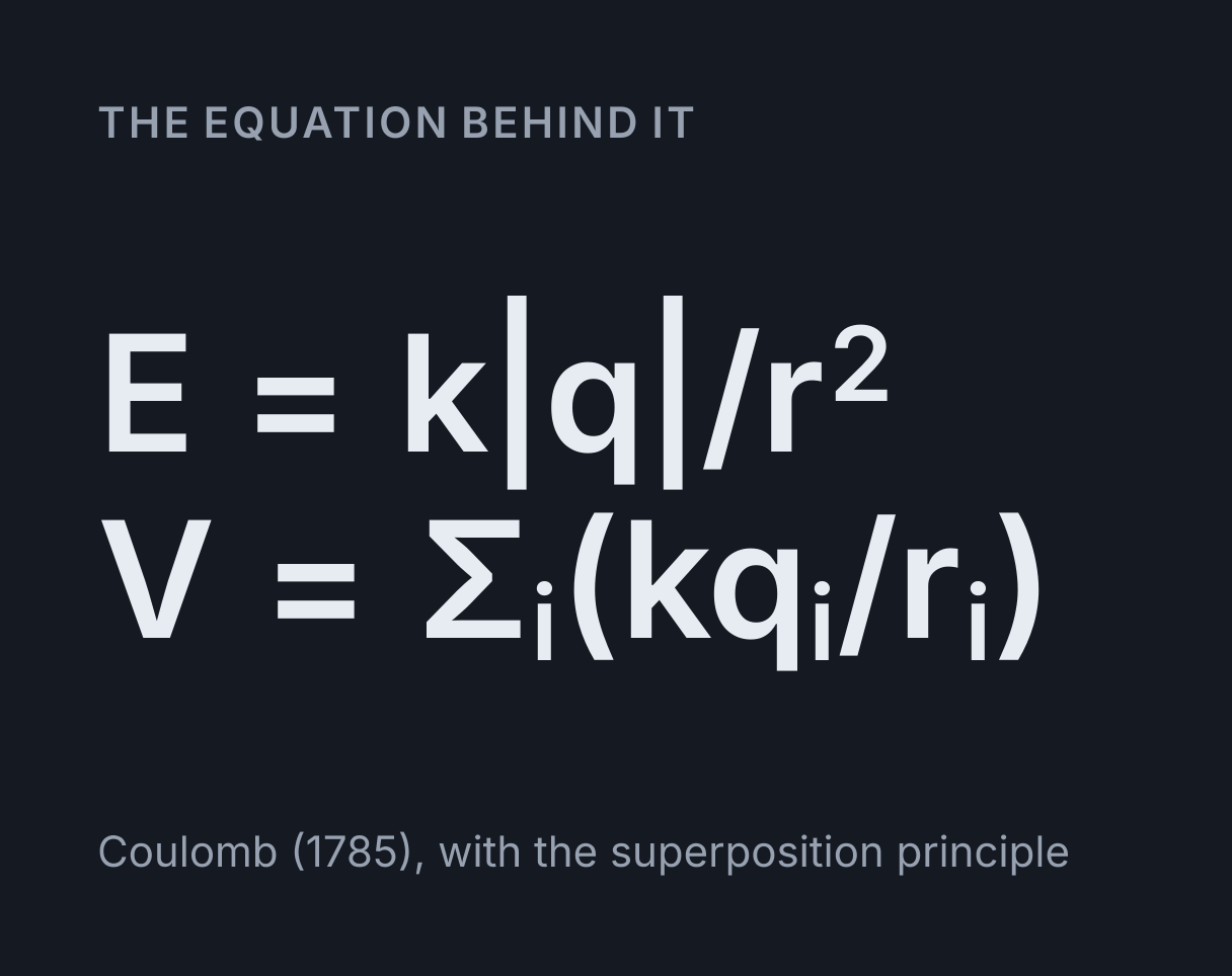
Coulomb (1785), with the superposition principle
How to find the electric field of several point charges
The electric field at any point is the vector sum of the fields of all the charges: each charge
contributes E = k|q|/r², pointing straight away from it if it is positive and
straight towards it if it is negative, with k = 1/(4πε₀) = 8.988 × 10⁹ N·m²/C².
The potential adds up the same way but as plain numbers with signs,
V = kq₁/r₁ + kq₂/r₂ + …, so a negative charge subtracts from it and no direction
is involved.
That is the superposition principle, and it is all this simulator does. Every number at the probe is Coulomb’s law worked out for one charge at a time and then added, which is why the table under the scene lists each charge’s share beside the total. The constant is Coulomb’s constant, computed from the CODATA 2022 vacuum permittivity.
Using the simulator
Drag a charge to move it, or pick it under Charges to set its size and position exactly. Add charges, up to 8, or start from one of the 6 arrangements under Start from. Drag the probe, or tap anywhere in the scene, to measure at that point. The readouts give the strength of the field in N/C, its direction measured anticlockwise from the +x axis, the potential in volts, and the force the field would exert on a +1 nC test charge placed there.
At the probe the scene draws each charge’s own field as a thin arrow, all to one scale and laid head to tail, and the total as a thicker arrow from the probe. The thin arrows end where the thick one does. That picture is the vector sum, and it is the part of the topic that arithmetic on magnitudes gets wrong.
Worked example: the field and potential of a dipole
Take charges of +2 nC and −2 nC 20 cm apart, the dipole the simulator opens with. At the
midpoint each is 10 cm away, so each field is
E = kq/r² = 8.9876 × 10⁹ × 2 × 10⁻⁹ / 0.10² = 1797.5 N/C, with k to five figures.
The positive charge’s field points away from it and the negative charge’s field points towards
it, which at the midpoint is the same way, so the two add: 3595 N/C, from the positive charge
towards the negative one. The potentials, +179.75 V and −179.75 V, cancel exactly, so the
potential there is 0 V.
Move the probe 10 cm up the bisector, to where the simulator opens. Each charge is now
√(10² + 10²) = 14.14 cm away, and the square of that distance, 200 cm², is twice
what it was, so each field is half as strong. Each field is now 898.8 N/C, one pointing up and
to the right at 45°, the other down and to the right at −45°. The vertical parts cancel and the
horizontal parts add, 2 × 898.8 × cos 45°, leaving 1271 N/C parallel to the axis,
pointing from the positive charge’s side to the negative’s. The potential is still 0 V,
because every point on the bisector is equally far from two equal and opposite charges.
The table under the scene gives the same figures to four significant figures, 1798 N/C for each charge at the midpoint and 3595 N/C for the two together, which is why the sum there looks one short: it is the unrounded 1797.5 that doubles.
The same sums reproduce textbook answers. Example 7.12 in OpenStax’s University Physics Volume 2 puts +3.0 nC and −3.0 nC 4.0 cm apart and asks for the potential at three points. With the charges at (0, 2) cm and (0, −2) cm, the probe at (0, 1), (0, −5) and (3, 2) cm reads 1798 V, −513.6 V and 359.5 V, which are the book’s 1.8 × 10³ V, −5.1 × 10² V and 3.6 × 10² V to the two significant figures it gives.
Zero field and zero potential are different things
The dipole’s bisector has zero potential and a strong field. The opposite happens between two like charges. Midway between two +2 nC charges 20 cm apart their fields are equal and opposite and cancel, so the field is zero, but their potentials are both +179.75 V and add to 359.5 V. Choose Two like charges under Start from and the probe lands on that point.
Unequal charges put the zero of the field somewhere less obvious. For +4 nC and −1 nC 20 cm apart it is on the axis, 20 cm beyond the −1 nC charge, where the larger charge is twice as far away: four times the charge at twice the distance gives the same field, 224.7 N/C each way. For unequal opposite charges the null point lies outside the pair, beyond the smaller one; for like charges it lies between them, nearer the smaller one. The potential at a null point is not zero either: 44.94 V at this one.
Field lines and equipotentials
A field line runs along the direction of the field at every point, so it starts on a positive charge and ends on a negative one, or leaves the picture. Two field lines never cross, because the field cannot point two ways at once. Away from the charges themselves, where lines begin and end, the one place lines meet is a point where the field is zero and has no direction at all, such as the midpoint of two like charges. Each charge here gets lines in proportion to its size, 8 per nanocoulomb until the scene holds more than 12 nC of one sign, when the count per nanocoulomb falls to keep the picture legible. A line that reaches the edge is carrying on beyond it.
An equipotential joins points at the same potential, and it always crosses the field lines at right angles. Moving along one takes no work, so the field can have no part along it. Following a field line takes you downhill in potential the whole way, which is why a positive charge released from rest sets off along the field and gains kinetic energy as its potential energy falls.
The equipotentials are drawn at equal steps of potential, and their spacing measures the field:
E ≈ ΔV/Δs. Around a single +2 nC charge the 250 V and 300 V rings are 1.2 cm
apart, a field of about 50 V ÷ 0.012 m ≈ 4200 N/C, while the 50 V and 100 V rings are 18 cm
apart, a field of about 280 N/C.
Why the lines are only a rough guide to strength here
In three dimensions the number of field lines through each square metre is proportional to the field, and textbooks read strength off line density for that reason. This picture is a flat slice through a three-dimensional field. Lines drawn evenly round a point charge in a plane move apart in proportion to r, so their density falls as 1/r, while the field falls as 1/r²: the lines thin out more slowly than the field does. The equipotentials are the reliable guide in a flat picture, and the probe gives the numbers.
What this simulator leaves out
- Size. Every charge is a point. A uniformly charged sphere has the same field outside it, but an object of any other shape does not, and nothing here has an inside.
- Matter. The charges sit in a vacuum. A conductor would rearrange its own charge in response, and a dielectric would weaken the field by its relative permittivity.
- Motion. The charges are held in place, although they push and pull on each other, and moving one changes the field everywhere at once. A real change travels outwards at the speed of light.
- The third dimension. All the charges lie in one plane, and only that plane is drawn. For two charges the field looks the same in every plane through the line joining them; for three or more it does so only when they lie on one line.
Common mistakes
- Adding field strengths as numbers. Fields add as vectors. At the dipole’s opening point the two fields are 898.8 N/C each and the total is 1271 N/C, not 1798.
- Treating zero potential as zero field. They are independent. Zero field between like charges comes with a potential of 359.5 V, and zero potential on a dipole’s bisector with a field of 3595 N/C at its midpoint.
- Forgetting that a negative charge’s field points towards it. The size
k|q|/r²takes no sign. The sign sets the direction, and in the potential it simply subtracts. - Leaving nanocoulombs and centimetres in the formula. k is in SI units, so 2 nC is 2 × 10⁻⁹ C and 10 cm is 0.10 m. Leaving the distance in centimetres puts the field out by a factor of 10⁴.
- Thinking a released charge follows the field line. The force on it is along the line, but a moving charge has momentum, so its path curves less than the line does and leaves it.
For the force between two charges, which is the field of one multiplied by the charge of the other, use the Coulomb’s law calculator. Two rows of opposite charges are a rough model of a parallel-plate capacitor, whose stored energy the capacitor energy calculator works out, and the solenoid magnetic field simulator does the same kind of sum for the magnetic field of a current.
Model and assumptions
- Method
- Exact expression, no time stepping
- Repeatability
- Deterministic. The same link gives the same numbers on any machine.
What it assumes
- Point charges held still in a vacuum, so the field and the potential are Coulomb’s law summed exactly over the charges, the field as a vector and the potential as a number.
- Every charge lies in the plane of the picture, so the field there has no part out of the plane and each field line drawn stays in it.
- The probe is an ideal test charge, which measures the field without pushing on the charges that make it.
Where it stops holding. Charged objects with size, conductors and dielectrics, where charge moves or polarises and a sum over fixed points no longer describes the field, and charges in motion, whose changes spread outwards at the speed of light rather than everywhere at once.
Numerical accuracy
No time stepping, so nothing accumulates. The readings at the probe and in the table are Coulomb’s law summed over the charges, exact to rounding. Two pictures are approximate by construction. Each field line is traced from its charge in short steps along the field direction, a fourth-order Runge-Kutta step in distance rather than time, and stays within a few micrometres of the true line wherever that line is known exactly. Each equipotential is found on a grid of points a few pixels apart, and every point where it crosses a grid line is then solved for exactly, so only the straight pieces joining those points are approximate: they stay within about two pixels of the true curve, the most where it bends sharply beside a small charge or close to a point where the field is zero.
Common questions
How do you find the electric field of several point charges?
Add the fields of the charges as vectors. Each charge contributes E = k|q|/r², pointing away from it if it is positive and towards it if it is negative, so split each field into x and y parts, add the parts, and combine them into one arrow. Midway between +2 nC and −2 nC charges 20 cm apart both fields are 1797.5 N/C and point towards the negative charge, so they add to 3595 N/C.
Can the electric field be zero where the potential is not?
Yes. Midway between two equal positive charges their fields are equal and opposite, so E = 0, but their potentials are both positive and add: for +2 nC charges 20 cm apart the potential there is 359.5 V. The reverse happens midway between +2 nC and −2 nC charges 20 cm apart, where the potentials cancel to V = 0 while the field is 3595 N/C.
Why do electric field lines cross equipotentials at right angles?
Because moving a charge along an equipotential takes no work, so the field can have no part along it. The field points the way the potential falls fastest, which is straight across the equipotentials, and its size is how fast the potential falls across them, E ≈ ΔV/Δs.
Does the spacing of field lines show how strong the field is?
Only roughly, in a flat picture like this one. In three dimensions the number of lines through each square metre is proportional to the field, but in a flat slice the lines from a point charge thin out as 1/r while its field falls as 1/r². The equipotentials are the reliable guide here: they are drawn at equal steps of potential, so where they crowd together the field is strong.
Where is the electric field zero for two unequal charges?
For opposite charges it is zero outside the pair, beyond the smaller charge; for like charges it is zero between them, nearer the smaller one. With +4 nC and −1 nC 20 cm apart the fields cancel 20 cm beyond the −1 nC charge, where the +4 nC charge is twice as far away and doubling the distance divides its field by four.