Hardy-Weinberg Calculator
Find p, q, p², 2pq and q² from any one known frequency or from genotype counts, then run a chi-square test of Hardy-Weinberg equilibrium on the counts.
Calculator
From 0 to 1, as 0.16.
Gives the expected number of each genotype.
- p, allele A The share of all copies of the gene that are A.
- 0.6
- q, allele a 1 − p, the share that are a.
- 0.4
- Dominant phenotype p² + 2pq: AA and Aa together, who look alike when A is dominant.
- 0.84
- Carriers among the dominant phenotype 2pq ÷ (p² + 2pq): the chance that someone with the dominant phenotype is Aa, when nothing else is known about them.
- 0.5714
| Genotype | Frequency | Percent | 1 in |
|---|---|---|---|
| AA p² | 0.36 | 36% | 2.78 |
| Aa 2pq | 0.48 | 48% | 2.08 |
| aa q² | 0.16 | 16% | 6.25 |
These follow from one number only by assuming Hardy-Weinberg equilibrium. To test it, enter genotype counts.
Working, step by step
- q² = 0.16
- q = sqrt(0.16) = 0.4
- p = 1 - 0.4 = 0.6
- p² = 0.6^2 = 0.36
- 2pq = 2 x 0.6 x 0.4 = 0.48
- p² + 2pq + q² = 0.36 + 0.48 + 0.16 = 1
Everything follows from p + q = 1 and the three squares. Only q² is a genotype you can see directly when A is dominant, which is why so many of these questions start with a square root.
Citing this tool
Last updated . Add the date you accessed it as well, which a citation of a page that can change asks for. If a specific result matters, cite the permalink from the tool’s share row instead of this page: it reproduces the exact parameters.
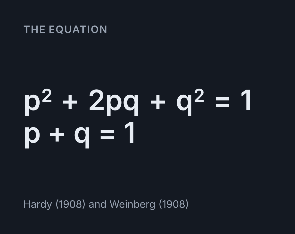
The equation
Hardy (1908) and Weinberg (1908)
The Hardy-Weinberg equation
The Hardy-Weinberg equation, p² + 2pq + q² = 1, gives the genotype
frequencies of a gene with two alleles in a population that is not evolving: if allele A
has frequency p and allele a has frequency q, with p + q = 1, then p² of the
population is AA, 2pq is Aa and q² is aa. This calculator finds all five numbers from any
one of them or from the dominant phenotype, or from counts of each genotype, and tests the
counts against those proportions with a chi-square test.
The proportions hold for a large population that mates at random, with no selection, mutation or migration, and with the same allele frequencies in males and females. One generation of random mating is enough to reach them, and after that they stay put. G. H. Hardy published the result in Science in July 1908, and the German physician Wilhelm Weinberg arrived at it independently the same year, which is why it carries both names.
Two ways in
One frequency takes whichever number a question gives you: p or q, one of the three genotype frequencies, or the share of the population with the dominant phenotype, as a frequency, a percentage or “1 in N”. Add a population size and it gives the expected number of each genotype as well. This mode assumes the population is in equilibrium, because one number cannot show that it is.
Genotype counts takes the number of AA, Aa and aa individuals in a sample. Counting alleles gives p and q without assuming anything, so the counts can then be tested: the calculator compares them with the counts equilibrium predicts, and reports χ², its p-value and an exact test that suits small samples.
Worked example: from the recessive phenotype
Suppose 16 percent of a population shows a recessive trait, a hypothetical figure and the
value loaded above. Those people are aa, so q² = 0.16.
q = √0.16 = 0.4p = 1 − 0.4 = 0.6p² = 0.6² = 0.362pq = 2 × 0.6 × 0.4 = 0.480.36 + 0.48 + 0.16 = 1, the check that nothing went astray
In a population of 1,000 that is 360 AA, 480 Aa and 160 aa. The 840 people with the dominant phenotype are not all alike: 480 of them, 0.48 ÷ 0.84 = 57.1 percent, carry the recessive allele without showing it.
How common are carriers of a rare recessive allele?
Take the square root of the frequency of the recessive phenotype to get q, then work out
2pq. For a recessive condition in 1 in 10,000 births, a round hypothetical figure,
q = √0.0001 = 0.01, p = 0.99 and
2pq = 2 × 0.99 × 0.01 = 0.0198: about 1 person in 50 is a carrier. For every
person with the condition there are 0.0198 ÷ 0.0001 = 198 carriers.
So nearly all copies of a rare recessive allele sit in people who do not show it: the share of them in carriers is p itself, 99 percent here. That is why selection against the recessive phenotype removes such an allele so slowly.
Worked example: testing genotype counts
Suppose a sample of 200, again hypothetical and the counts loaded under Genotype counts, holds 90 AA, 80 Aa and 30 aa.
-
Count the alleles. Of the 400 copies of the gene, 2 × 90 + 80 = 260 are A, so
p = 260 ÷ 400 = 0.65andq = 0.35. -
Expected counts:
200 × 0.65² = 84.5AA,2 × 200 × 0.65 × 0.35 = 91Aa and200 × 0.35² = 24.5aa. -
χ² = (90 − 84.5)²/84.5 + (80 − 91)²/91 + (30 − 24.5)²/24.5, which is0.3580 + 1.3297 + 1.2347 = 2.9224. -
With 1 degree of freedom the critical value at 0.05 is 3.841. 2.9224 is below it, and
p = 0.0874: not significant.
The sample has fewer heterozygotes than equilibrium predicts, 80 against 91, but not so few that chance is an unlikely explanation. The exact test agrees, with p = 0.0886. Keep the same p and move heterozygotes into the homozygote classes, 50 AA, 30 Aa and 20 aa in a sample of 100, and χ² rises to 11.6 with p = 0.000658: significant.
Why the test has one degree of freedom
There are three genotypes, but the expected counts are made to add up to the sample size,
which takes away one degree of freedom, and p is estimated from the same counts, which
takes away another: 3 − 1 − 1 = 1. It is the general rule for goodness of
fit, the number of classes less one less the number of parameters estimated from the data,
as the NIST/SEMATECH e-Handbook of Statistical Methods states it.
Using 2 degrees of freedom, as if p had been known in advance, raises the critical value from 3.841 to 5.991 and makes real departures harder to detect. If p really does come from somewhere else, 2 is right, and the chi-square calculator runs that test against the ratio p²:2pq:q².
Small samples and rare alleles: the exact test
The chi-square p-value comes from an approximation that needs every expected count to be
reasonably large, and the usual rule of thumb is at least 5. With a rare allele the
expected number of rare homozygotes is tiny, and the approximation fails. In a sample of
46 AA, 3 Aa and 1 aa, q = 0.05, so only
50 × 0.05² = 0.125 aa individuals are expected. The single one observed
contributes 6.125 to χ² = 6.787, and p = 0.00918 looks
decisive.
The exact test needs no approximation. Computed as Wigginton, Cutler and Abecasis (2005)
describe, it works out the probability of every possible number of heterozygotes given the
allele counts, and adds up those no more likely than the one observed. Here that gives
p = 0.0994, not significant at 0.05. Their paper showed that the chi-square
test can reject a population that is in equilibrium far too often when an allele is
rare, even in large samples, while the exact test never does so more often than its
significance level allows. The calculator reports both, and says which to trust when an
expected count is below 5 or the two disagree.
What a departure from equilibrium means
A significant χ² says the counts are unlikely under Hardy-Weinberg proportions. It does not say why, but the direction narrows it down, and F, one minus the ratio of observed to expected heterozygotes, gives the direction: positive for too few, negative for too many. With two alleles, χ² is exactly N × F², so the test asks whether F is zero.
Too few heterozygotes is what inbreeding produces. It is also what a sample pooled from populations with different allele frequencies shows, the Wahlund effect, and what genotyping that misreads heterozygotes as homozygotes leaves behind. Too many can come from selection that favours heterozygotes before the sample was taken, or from allele frequencies that differ between the sexes.
What this calculator does not cover
- Crosses between two known parents. The equation describes a whole population mating at random. For the offspring of one cross, use the Punnett square calculator.
- More than two alleles. The ABO blood group has three, which gives six
genotypes and
(p + q + r)² = 1, and a test with more degrees of freedom. - X-linked genes. Males carry one copy, so a recessive X-linked trait appears in a fraction q of males but only q² of females.
- Phenotype counts under complete dominance. AA and Aa look alike, so their counts cannot be told apart, p cannot be counted and the test cannot be run. It needs genotyping, or alleles that are codominant.
- Change over time. Drift, selection and migration move allele frequencies between generations. The equation describes one generation, not the path.
Common mistakes
- Taking the square root of the dominant phenotype. It is p² + 2pq, not a
square. Subtract it from 1 to get q², and take the root of that: a dominant phenotype of
91 percent gives
q² = 0.09andq = 0.3. - Confusing q with q². The share of people showing a recessive trait is q², a genotype frequency. The allele frequency q is its square root, and larger: 0.4 against 0.16 in the example above.
- Dropping the 2 in 2pq. There are two ways to be a heterozygote, A from the mother and a from the father or the other way round.
- Testing numbers made by assuming equilibrium. Genotype counts worked out from q² fit Hardy-Weinberg proportions by construction. Only counts of real individuals can test them.
- Using 2 degrees of freedom. When p comes from the same counts, the test has 1, and the critical value at 0.05 is 3.841.
- Reading “not significant” as proof. It means the counts are consistent with equilibrium. A small sample is consistent with a great deal.
Common questions
How do you calculate p and q from genotype counts?
Count the alleles: p = (2 × AA + Aa) ÷ 2N and q = 1 − p, because each AA individual carries two copies of A and each Aa carries one. For 90 AA, 80 Aa and 30 aa, N = 200, so p = 260 ÷ 400 = 0.65 and q = 0.35. Counting needs no assumption about the population; it is the genotype frequencies p², 2pq and q² that depend on equilibrium.
How do you find the carrier frequency from the recessive phenotype?
Take the square root of the recessive phenotype’s frequency to get q, then work out 2pq with p = 1 − q. For a hypothetical recessive trait in 1 in 10,000 people, q = 0.01, p = 0.99 and 2pq = 0.0198, or about 1 carrier in every 50 people. The step from q² to q assumes Hardy-Weinberg equilibrium, which a single frequency cannot check.
How many degrees of freedom does a Hardy-Weinberg chi-square test have?
One, for a gene with two alleles. There are three genotype classes; one degree of freedom goes because the expected counts are scaled to the sample size, and a second because p is estimated from the same counts. The critical value at 0.05 is therefore 3.841, not the 5.991 that 2 degrees of freedom would give.
What does it mean if a population is not in Hardy-Weinberg equilibrium?
That at least one of the conditions behind the proportions fails, though a test cannot say which. Too few heterozygotes points to inbreeding or to a sample pooled from populations with different allele frequencies, and too many can come from selection that favours heterozygotes. In real data, genotyping that misses heterozygotes can also produce a shortage. A result that is not significant is not proof of equilibrium either, since a small sample can miss a small departure.
What are the conditions for Hardy-Weinberg equilibrium?
Random mating in a large population, with no selection, mutation or migration, for a gene in a diploid, sexually reproducing species whose generations do not overlap and whose allele frequencies are the same in both sexes. Under those conditions one generation of random mating gives genotype frequencies of p², 2pq and q², and they then stay the same from one generation to the next.