Chi-Square Calculator
Chi-square test for counts: goodness of fit to a ratio such as 9:3:3:1, or independence in a contingency table, with χ², degrees of freedom and p-value.
Calculator
The ratio can be in any units: 9, 3, 3, 1, or proportions, or expected counts. It is scaled so the expected counts add up to the observed total.
- χ² The sum of (O − E)² / E over every cell. It is 0 for a perfect match and grows with the size of the differences.
- 0.47
- Degrees of freedom Categories minus 1, minus any parameters estimated from these counts.
- 3
- p-value The probability of a χ² at least this large if the null hypothesis were true. It is not the probability that the hypothesis is true.
- 0.925
- Critical value, α = 0.05 The χ² that leaves exactly α in the upper tail at these degrees of freedom. A χ² at or above it is significant.
- 7.815
Not significant at α = 0.05. χ² = 0.47 is below the critical value of 7.815, so do not reject the null hypothesis that the counts follow the expected ratio. If it were true, a χ² at least this large would turn up with probability 0.925: the data are consistent with it, which is not the same as proving it.
| Category | O | E | O − E | (O − E)² | (O − E)² / E |
|---|---|---|---|---|---|
| Round yellow | 315 | 312.75 | 2.25 | 5.0625 | 0.016187 |
| Wrinkled yellow | 101 | 104.25 | −3.25 | 10.563 | 0.10132 |
| Round green | 108 | 104.25 | 3.75 | 14.063 | 0.13489 |
| Wrinkled green | 32 | 34.75 | −2.75 | 7.5625 | 0.21763 |
| Total | 556 | 556 | 0.47002 |
| α | 0.10 | 0.05 | 0.025 | 0.01 | 0.005 | 0.001 |
|---|---|---|---|---|---|---|
| χ² | 6.251 | 7.815(the level chosen) | 9.348 | 11.345 | 12.838 | 16.266 |
- χ² distribution, 3 degrees of freedom
- Critical value at α = 0.05
- χ² = 0.47
Working
- N = 315 + 101 + 108 + 32 = 556
- E for Round yellow = 556 x 9 / 16 = 312.75
- E for Wrinkled yellow = 556 x 3 / 16 = 104.25
- E for Round green = 556 x 3 / 16 = 104.25
- E for Wrinkled green = 556 x 1 / 16 = 34.75
- χ² = 0.016187 + 0.10132 + 0.13489 + 0.21763 = 0.47002
- degrees of freedom = 4 - 1 = 3
- p-value = P(χ² ≥ 0.47002) = 0.92543
- critical value at α = 0.05 = 7.8147
- 0.47002 < 7.8147, so p > 0.05: not significant at α = 0.05
Citing this tool
Last updated . Add the date you accessed it as well, which a citation of a page that can change asks for. If a specific result matters, cite the permalink from the tool’s share row instead of this page: it reproduces the exact parameters.
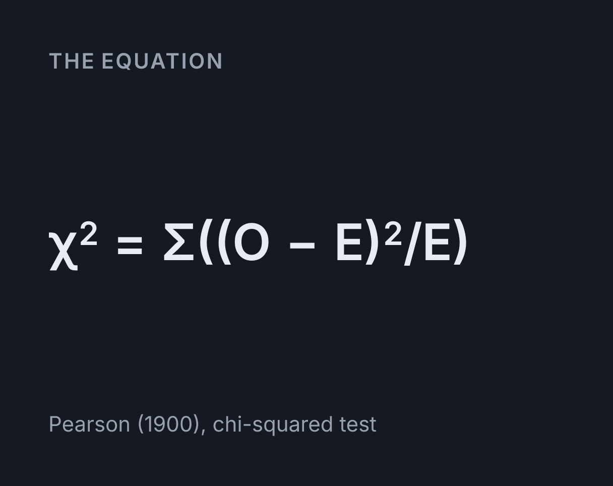
The equation
Pearson (1900), chi-squared test
What a chi-square test tells you
A chi-square test measures how far a set of observed counts sits from the counts a hypothesis predicts. For each category, subtract the expected count from the observed one, square the difference, divide by the expected count, and add the results: χ² = Σ (O - E)² / E. The p-value is then the probability of a χ² at least that large if the hypothesis were true, read from the chi-square distribution with the right number of degrees of freedom.
Dividing by E is what makes the differences comparable. A miss of a few seeds matters far more in a class where 35 were expected than in one where 313 were: in Mendel’s count below, a difference of 2.75 against an expected 34.75 contributes 0.218 to χ², while a difference of 2.25 against 312.75 contributes only 0.016.
Which test to choose
- Goodness of fit asks whether one set of counts follows a ratio stated in advance, such as 9:3:3:1 from a dihybrid cross, 3:1 from a monohybrid one, or equal numbers on each face of a die. Each expected count is the total times that category’s share of the ratio, and the degrees of freedom are the number of categories minus 1, minus one more for every parameter estimated from the same counts.
- Contingency table asks whether two ways of classifying the same individuals are independent. Each expected count is its row total times its column total divided by the grand total, and the degrees of freedom are
(rows - 1) × (columns - 1). - p-value from χ² takes a statistic you already have and gives its p-value, its lower tail and the critical values, for up to 1,000 degrees of freedom: the job a printed chi-square table does, without the gaps between its columns.
All three work on counts of individuals. For measurements such as lengths, masses or reaction times, the spread and the uncertainty of the mean come from the standard deviation calculator, and a trend between two measured variables from the linear regression calculator.
Worked example: Mendel’s 9:3:3:1 dihybrid cross
Mendel crossed peas with round yellow seeds with peas with wrinkled green seeds, let the 15 hybrid plants fertilise themselves, and counted 556 seeds: 315 round yellow, 101 wrinkled yellow, 108 round green and 32 wrinkled green. These are the counts the calculator opens with. If seed shape and colour are each inherited with one dominant allele and assort independently, they should fall in the ratio 9:3:3:1.
- Expected counts:
556 × 9/16 = 312.75,556 × 3/16 = 104.25twice, and556 × 1/16 = 34.75. - Contributions:
2.25²/312.75 = 0.0162,3.25²/104.25 = 0.1013,3.75²/104.25 = 0.1349and2.75²/34.75 = 0.2176. χ² = 0.470on4 - 1 = 3degrees of freedom.- The critical value at α = 0.05 is 7.815, and the p-value is 0.925.
So the counts are entirely consistent with 9:3:3:1, and a report would read χ²(3, N = 556) = 0.47, p = .93. A p-value that large does not prove the ratio. It says only that differences this size turn up by chance most of the time when the ratio is exactly right.
Worked example: do the two traits assort independently?
The same 556 seeds can be laid out as a 2 × 2 table, round or wrinkled by yellow or green, which asks a narrower question: is colour independent of shape? The row totals are 423 round and 133 wrinkled, the column totals 416 yellow and 140 green, so the expected number of round yellow seeds is 423 × 416 / 556 = 316.49. The four contributions add up to χ² = 0.116 on 1 degree of freedom, and the p-value is 0.733.
The two tests ask different things of one data set. The contingency table uses the observed proportions of round and of yellow, so it would pass even if the ratio of round to wrinkled were far from 3:1. The 9:3:3:1 test fixes both proportions in advance as well, which is why it has three degrees of freedom: once the total is known, three of the four counts can still vary freely, and the fourth is whatever is left.
What a significant result looks like
Suppose a test cross, AaBb × aabb, gives 44, 6, 7 and 43 offspring in the four classes where independent assortment predicts 25 of each. Then χ² = (19² + 19² + 18² + 18²) / 25 = 54.8 on 3 degrees of freedom, and the p-value is 7.57 × 10⁻¹². The hypothesis is rejected, and the pattern says why: the two parental classes are far too common, which is what linked genes produce. The 13 recombinants in 100 would put the genes about 13 map units apart.
Degrees of freedom can flip a verdict. Suppose a sample of 100 individuals has 30 AA, 40 Aa and 30 aa. The allele frequency estimated from those counts is 0.5, so Hardy-Weinberg proportions predict 25, 50 and 25, and χ² = 1 + 2 + 1 = 4. Because the frequency was estimated from the same counts, the test has 3 - 1 - 1 = 1 degree of freedom and a p-value of 0.0455, significant at 0.05. Forget the estimated parameter and the same χ² on 2 degrees of freedom gives 0.135, which is not. The calculator has a box for the number of parameters estimated for exactly this reason.
Critical values of the chi-square distribution
A result is significant at level α when χ² is at or above the critical value for its degrees of freedom. The table runs to 100 degrees of freedom; the calculator gives any value up to 1,000.
| Degrees of freedom | 0.10 | 0.05 | 0.025 | 0.01 | 0.005 | 0.001 |
|---|---|---|---|---|---|---|
| 1 | 2.706 | 3.841 | 5.024 | 6.635 | 7.879 | 10.828 |
| 2 | 4.605 | 5.991 | 7.378 | 9.210 | 10.597 | 13.816 |
| 3 | 6.251 | 7.815 | 9.348 | 11.345 | 12.838 | 16.266 |
| 4 | 7.779 | 9.488 | 11.143 | 13.277 | 14.860 | 18.467 |
| 5 | 9.236 | 11.070 | 12.833 | 15.086 | 16.750 | 20.515 |
| 6 | 10.645 | 12.592 | 14.449 | 16.812 | 18.548 | 22.458 |
| 7 | 12.017 | 14.067 | 16.013 | 18.475 | 20.278 | 24.322 |
| 8 | 13.362 | 15.507 | 17.535 | 20.090 | 21.955 | 26.124 |
| 9 | 14.684 | 16.919 | 19.023 | 21.666 | 23.589 | 27.877 |
| 10 | 15.987 | 18.307 | 20.483 | 23.209 | 25.188 | 29.588 |
| 15 | 22.307 | 24.996 | 27.488 | 30.578 | 32.801 | 37.697 |
| 20 | 28.412 | 31.410 | 34.170 | 37.566 | 39.997 | 45.315 |
| 25 | 34.382 | 37.652 | 40.646 | 44.314 | 46.928 | 52.620 |
| 30 | 40.256 | 43.773 | 46.979 | 50.892 | 53.672 | 59.703 |
| 40 | 51.805 | 55.758 | 59.342 | 63.691 | 66.766 | 73.402 |
| 50 | 63.167 | 67.505 | 71.420 | 76.154 | 79.490 | 86.661 |
| 100 | 118.498 | 124.342 | 129.561 | 135.807 | 140.169 | 149.449 |
The figures agree with the NIST/SEMATECH e-Handbook of Statistical Methods to the three decimals it prints, except once: at 8 degrees of freedom and 0.001 it prints 26.125, where the value is 26.1245 and rounds to 26.124.
The lower tail matters too. A χ² far smaller than its degrees of freedom means the counts sit closer to the hypothesis than chance usually allows, which can point to data selected or adjusted to fit. Mendel’s 9:3:3:1 counts have a lower tail of 0.0746, and Fisher (1936) argued, over all of Mendel’s experiments together, that his results fitted his ratios too well.
Small expected counts and Yates’ correction
The p-value comes from the chi-square distribution, which is an approximation to the true sampling distribution of the statistic, and it fails when expected counts are small. The guideline usually traced to Cochran (1954) allows no expected count below 1 and no more than 20 percent of them below 5; the calculator warns when a table breaks it. Combining categories or collecting more data fixes the problem, and for a 2 × 2 table Fisher’s exact test avoids the approximation altogether.
For a 2 × 2 table the calculator also gives Yates’ continuity correction, which reduces each |O - E| by 0.5 before squaring. On Mendel’s table it lowers χ² from 0.116 to 0.0513 and raises the p-value from 0.733 to 0.821. The correction makes the test more conservative and is disputed: many statisticians prefer the uncorrected statistic, or an exact test when counts are small, so report which one you used.
Common mistakes
- Using percentages or proportions instead of counts. χ² grows with the number of observations for the same proportions: Mendel’s proportions give 0.470 at 556 seeds, 0.085 at 100 and 4.70 at 5,560.
- The wrong degrees of freedom. It is categories minus 1 for a goodness-of-fit test, not the number of categories, and one fewer again for every parameter estimated from the data.
- Dividing by the observed count. The divisor is always E, the count the hypothesis predicts.
- Reading “not significant” as proof. Failing to reject a hypothesis is not evidence that it is true, especially with a small sample.
- Counting an individual twice. Each observation must fall in exactly one cell. Before and after measurements on the same people need McNemar’s test instead.
- Reading the wrong column of a printed table. Tables are laid out either by the upper tail, α, or by the cumulative probability, 1 - α. The 0.05 column here is the one some books head 0.95.
What this calculator leaves out
It runs Pearson’s test, with Yates’ correction as its 2 × 2 variant, and no other: not Fisher’s exact test, the G-test, McNemar’s test for paired data, or the cell-by-cell comparisons that follow a significant table. Its p-value is the chi-square approximation, which is why it warns about small expected counts. It also takes the expected ratio as given: the Punnett square calculator works one out from a cross, and the Hardy-Weinberg calculator from a population.
Common questions
How do you calculate chi-square?
Subtract each expected count from the observed count, square the difference, divide by the expected count, and add the results over every category: χ² = Σ (O − E)² / E. Mendel’s 315, 101, 108 and 32 seeds against a 9:3:3:1 ratio have expected counts of 312.75, 104.25, 104.25 and 34.75, which give χ² = 0.470.
How many degrees of freedom does a chi-square test have?
The number of categories minus 1 for a goodness-of-fit test, less one more for each parameter estimated from the same counts, and (rows − 1) × (columns − 1) for a contingency table. So a 9:3:3:1 test has 3, a 2 × 2 table has 1, and a Hardy-Weinberg test on three genotypes with the allele frequency estimated from the sample has 3 − 1 − 1 = 1.
What does the p-value of a chi-square test mean?
It is the probability of a χ² at least as large as yours if the null hypothesis were true. At or below the significance level, usually 0.05, the counts differ from the expected ones by more than chance usually produces, and the hypothesis is rejected. Above it they are consistent with the hypothesis, which is not the same as proving it.
What is the critical value of chi-square at 0.05?
It depends on the degrees of freedom: 3.841 for 1, 5.991 for 2, 7.815 for 3, 9.488 for 4 and 11.070 for 5. A χ² at or above the critical value is significant at 0.05. The table on this page runs to 100 degrees of freedom, and the calculator gives the value for up to 1,000.
What if an expected count is less than 5?
Then the p-value may be unreliable, because the chi-square distribution only approximates the statistic and the approximation fails when expected counts are small. A widely used guideline, usually traced to Cochran (1954), allows no expected count below 1 and no more than 20 percent below 5. Past that, combine categories or collect more data; for a 2 × 2 table, Fisher’s exact test is the usual alternative.