Motion Graphs Simulator
Motion graphs simulator: watch distance-time, velocity-time and acceleration-time graphs draw as a cart moves, with the gradients and areas read out live.
Simulator
Drag across the graphs to read any moment, or use the arrow keys: left and right step a tenth of a second, up and down jump between stages. Space plays and pauses.
A cart on a straight track runs 5 stages over 16 s and ends 36 m forwards of the start, after 36 m of travel. At t = 0 s it is in stage 1, momentarily at rest: at the start, with a velocity of 0 m/s and an acceleration of 1 m/s². Below the track, the position-time, velocity-time and acceleration-time graphs are drawn up to this moment, with the tangent to the position-time graph and the areas under the other two shaded. Dots on the track mark where the cart was every 1 s.
- Velocity (gradient of x-t) The gradient of the position-time graph at this moment, v = dx/dt. Within a stage it is v = u + at, and a negative value means the cart is moving backwards.
- 0 m/s
- Acceleration (gradient of v-t) The gradient of the velocity-time graph, a = dv/dt, which is constant through each stage. At the instant one stage hands over to the next, it gives the stage that is starting.
- 1 m/s²
- Displacement (area under v-t) The area between the velocity-time graph and the time axis from 0 to now, with area below the axis counted as negative. Each stage adds s = ½(u + v)t, and the total is the height of the position-time graph, because the cart starts at 0 m.
- 0 m
- Distance travelled The area under the speed-time graph, |v| against t. It matches the displacement until the cart turns round, then keeps growing while the displacement falls.
- 0 m
- Change in velocity (area under a-t) The area under the acceleration-time graph from 0 to now. Each stage adds a × t, and the total is v − u, the velocity now less the starting velocity.
- 0 m/s
Start from
Over the whole run
- Total displacement The signed area under the whole velocity-time graph: how far from the start the run ends, and on which side.
- 36 m
- Total distance The area under the whole speed-time graph: every metre covered, whichever way the cart was going.
- 36 m
- Average velocity Total displacement over total time, 36 m in 16 s: the gradient of a straight line from the first point of the position-time graph to the last.
- 2.25 m/s
- Average speed Total distance over total time, 36 m in 16 s. It equals the average velocity only when the cart never moves backwards.
- 2.25 m/s
- Distance travelled
- Displacement from the start
Citing this tool
Last updated . Add the date you accessed it as well, which a citation of a page that can change asks for. If a specific result matters, cite the permalink from the tool’s share row instead of this page: it reproduces the exact parameters.
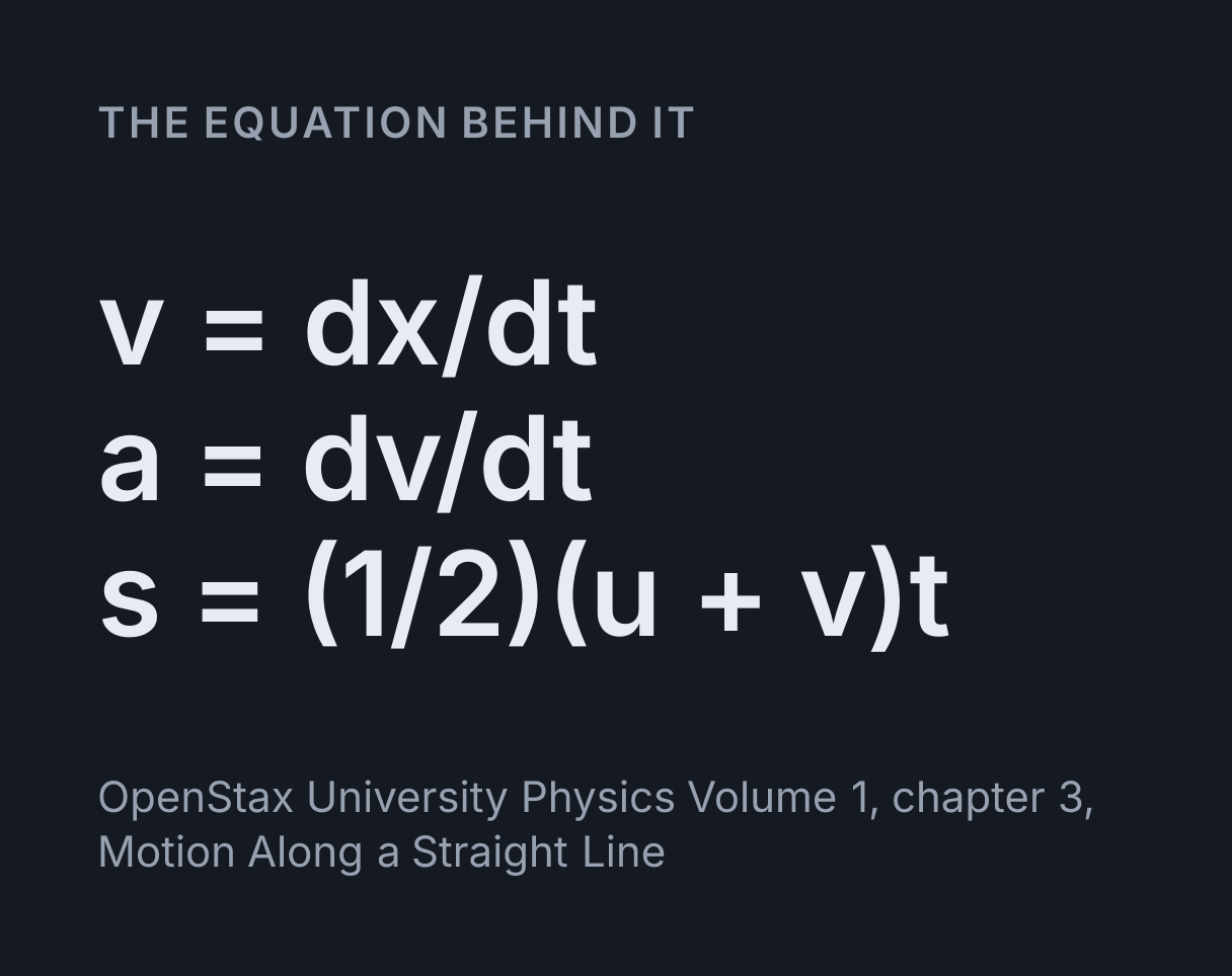
The equation
OpenStax University Physics Volume 1, chapter 3, Motion Along a Straight Line
What are motion graphs?
Motion graphs are the three graphs that describe something moving in a straight line: position
against time, velocity against time and acceleration against time. Every graph after the first is
the gradient of the one above it, and the area under it is the change in that one. The gradient of
the position-time graph is the velocity, v = dx/dt; the gradient of the velocity-time
graph is the acceleration, a = dv/dt; and the area under the velocity-time graph is
the displacement, which for a stretch of constant acceleration is a trapezium,
s = ½(u + v)t.
This motion graphs simulator runs a cart along a straight track through up to five stages, each with its own duration and constant acceleration, and draws all three graphs as the cart moves. Because the acceleration is constant within each stage, every graph is exact: straight lines and parabolas on the position-time graph, straight lines on the velocity-time graph and flat steps on the acceleration-time graph. The readouts give the gradients and the areas at the moment shown, so each link between the graphs can be checked number by number rather than taken on trust.
Using the simulator
Choose one of the five preset journeys, or build your own a stage at a time. The starting velocity is how fast the cart is already moving at t = 0, with forwards positive. Each stage has a duration and an acceleration: 0 for constant velocity, positive to push the cart forwards and negative to push it backwards. A stage always starts at the position and velocity the one before it ended with, so the velocity never jumps.
Play runs the journey in real time, and the speed control slows it down or speeds it up. The scrubber under the scene moves through it by hand. You can also drag across the graphs to read them at any moment, or select the scene and use the arrow keys: left and right move the clock a tenth of a second, up and down jump to the start of the next or the previous stage, and Home and End go to either end of the run.
The cart carries two arrows, its velocity and its acceleration, each in the colour of its own graph. When they point the same way the cart is speeding up, and when they point opposite ways it is slowing down. The dots it leaves on the track mark where it was at each second, or every few seconds on a long run, like the dots a ticker timer prints on paper tape: wide gaps where it was fast, close ones where it was slow. On the position-time graph the dashed line is the tangent at the current moment, and on the other two graphs the shading is the area under the line so far.
The first readouts are for the moment the clock shows: the velocity, as the gradient of the position-time graph; the acceleration, as the gradient of the velocity-time graph; the displacement, as the area under the velocity-time graph; the distance travelled; and the change in velocity, as the area under the acceleration-time graph. Above the distance plot, the whole-run readouts give the total displacement and distance and the average velocity and speed.
Worked example: the stop-and-start journey
The simulator opens on a five-stage journey from rest: speed up, cruise, brake to a stop, wait, and set off again. Every area under its velocity-time graph is a whole number of metres, which makes it easy to check by hand.
-
Stage 1, 4 s at 1 m/s² from rest:
v = u + at = 0 + 1 × 4 = 4 m/s, and the area under the velocity-time graph is a triangle,½ × 4 × 4 = 8 m. -
Stage 2, 4 s at a steady 4 m/s: the area is a rectangle,
4 × 4 = 16 m, so after 8 s the cart is8 + 16 = 24 mfrom the start. -
Stage 3, 2 s at −2 m/s²:
v = 4 + (−2) × 2 = 0 m/s, and the triangle under the graph is½ × 2 × 4 = 4 m, which leaves the cart at 28 m. - Stage 4, 2 s at rest: no area at all, and the position-time graph runs flat at 28 m.
- Stage 5, 4 s at 1 m/s² again: back up to 4 m/s, and another 8 m.
-
Altogether
8 + 16 + 4 + 0 + 8 = 36 min 16 s, so the average velocity is36 / 16 = 2.25 m/s, the gradient of a straight line from the first point of the position-time graph to the last.
The gradient readout shows the difference between average and instantaneous velocity. Scrub to
t = 2 s and the cart is ½ × 1 × 2² = 2 m from the start, so its average velocity so far
is 1 m/s, but the tangent there has a gradient of 2 m/s, which is the velocity readout. Halfway
through the braking, at t = 9 s, the cart is at 24 + 4 × 1 − ½ × 2 × 1² = 27 m, moving
at 2 m/s with an acceleration of −2 m/s². Each stage is one constant-acceleration problem, and the
kinematics calculator solves any of them with the SUVAT
equations.
Reading a distance-time graph
The top graph is the position-time graph: how far the cart is from where it started, against time. School courses often call it a distance-time graph, because for a journey in one direction the distance from the start and the distance travelled are the same thing. Its gradient is the velocity. A straight line means constant velocity, and the steeper the line, the faster the cart. A flat line means the cart is stationary. A curve means the velocity is changing: it bends upwards as the cart speeds up and levels off as it slows down.
On a curve, the velocity at one instant is the gradient of the tangent there, the straight line through that point with the same steepness as the curve, which the simulator draws dashed. By hand that means drawing a tangent and reading two points far apart on it; the readout gives the exact value to compare. The gradient of a curve at a point is exactly what a derivative is, and the derivative and tangent line explorer draws the tangent to any function in the same way.
A line sloping down means the cart is heading back towards the start, with a negative velocity. That is where the name distance-time graph starts to mislead, because the distance travelled can never go down, so a graph that falls is really showing displacement. The plot under the scene draws the two together, and they part company at the moment the cart turns round.
Reading a velocity-time graph
The middle graph is the velocity-time graph, and its gradient is the acceleration. A line sloping
up is a positive acceleration, a flat line is constant velocity with no acceleration, and a line
sloping down is a negative acceleration. In the opening journey the braking stage drops from 4 m/s
to rest in 2 s, a gradient of (0 − 4) / 2 = −2 m/s².
The height of the line is the velocity, so where the line is below the time axis, the cart is moving backwards. A straight line that crosses the axis is a cart that slows to a stop and reverses without any change in its acceleration. Velocity cannot jump, so a velocity-time graph is always one unbroken line, and its corners are the moments the acceleration changes.
The area under a velocity-time graph
The area between the velocity-time graph and the time axis is the displacement. For constant
acceleration that area is a trapezium, the average of the starting and final velocities times the
time, s = ½(u + v)t, which is the same as s = ut + ½at². The simulator
shades the area up to the current moment and reads it out, and it always matches the height of the
position-time graph, because the cart starts at 0 m.
Area below the time axis counts as negative, because it is motion backwards. In the there and back
preset the cart is sent off at 4 m/s and slowed at 1 m/s², so it stops after 4 s and comes back.
The triangle above the axis is ½ × 4 × 4 = 8 m and the one below it is −8 m, so after
8 s the displacement is zero. The distance travelled is the area under the speed-time graph
instead, with both triangles counted as positive, which comes to 16 m.
Under a curved velocity-time graph the area has to be found by counting squares or by adding up thin strips, which is what integration does exactly, and the Riemann sum and integral explorer shows the strips closing in on the true area. Here every velocity-time graph is made of straight lines, so the trapeziums give the exact area.
The acceleration-time graph
The bottom graph is the acceleration against time. With one constant acceleration in each stage it
is a row of flat steps that jump at the boundaries between stages. The area under it is the change
in velocity: the first step of the opening journey, 1 m/s² high and 4 s long, adds
1 × 4 = 4 m/s, and the braking step takes it away again, −2 × 2 = −4 m/s.
The readout of that area is always the velocity now less the starting velocity.
A fall in a vacuum is the simplest acceleration-time graph there is: one flat line at g. Taking
downwards as positive, a single stage of 2 s at 9.8 m/s² from rest falls
½ × 9.8 × 2² = 19.6 m and reaches 9.8 × 2 = 19.6 m/s. Air resistance
changes that, and the free fall calculator works out the
same kind of drop with drag included.
There and back: zero velocity is not zero acceleration
The there and back preset is one stage, not two. The cart starts at 4 m/s and its acceleration is
−1 m/s² from start to finish. It slows, stops for an instant at 4 s, and comes back, speeding up
backwards to −4 m/s at 8 s. The position-time graph is a single upside-down parabola peaking at
4² / (2 × 1) = 8 m, the velocity-time graph is one straight line crossing the time
axis, and the acceleration-time graph is flat at −1 m/s² all the way along.
So at the moment the cart is stopped, its acceleration is still −1 m/s². A ball thrown straight up is the same: at the top its velocity is zero and its acceleration is still g, downwards, which is why it comes back. If its acceleration were zero at the top, it would stay there.
The same run separates velocity from speed. Its average velocity over the 8 s is
0 / 8 = 0 m/s, because the cart ends where it started, while its average speed is
16 / 8 = 2 m/s. It also shows that a negative acceleration only slows the cart while
its velocity is positive: for the last 4 s the same −1 m/s² speeds it up.
What this model leaves out
- Gradual changes in acceleration. Here the acceleration jumps from one value to the next at each boundary. A real vehicle takes a moment to change it, so its acceleration-time graph has sloping sides and its velocity-time graph has rounded corners. The rate of change of acceleration is called jerk, and it is what passengers feel as a lurch.
- Acceleration that varies within a stage. Each stage has one constant acceleration. Air resistance grows with speed, so a falling object’s acceleration shrinks towards zero as it nears terminal velocity, which gives a curved velocity-time graph that a run of stages can only approximate.
- The forces behind the motion. The graphs describe the motion without saying what causes it. The acceleration comes from the resultant force, a = F/m, which the free-body diagram maker finds from the forces acting on an object.
- Motion in more than one direction. The track is straight, so position, velocity and acceleration are single numbers with a sign. A thrown ball moving across and up at once needs a separate set of graphs for each direction.
- Measurement. Real motion graphs come from light gates, ticker timers, motion sensors or video, with noise and a finite sampling rate. Here every value is exact, and stage durations move in steps of 0.1 s.
Common mistakes
- Reading the gradient of the wrong graph. The gradient of a position-time graph is velocity, but the gradient of a velocity-time graph is acceleration. A steep velocity-time graph means a large acceleration, not a high speed.
- Reading the height of a position-time graph as the speed. The height is where the cart is; the speed is how steep the line is. At 11 s in the opening journey the graph is at 28 m, its highest so far, while the cart is standing still.
- Treating a flat line the same on every graph. Flat on a position-time graph means stationary. Flat on a velocity-time graph means constant velocity, which can be fast. Flat at zero on an acceleration-time graph means the velocity is not changing.
- Thinking zero velocity means zero acceleration. At the turning point of the there and back run the cart is stopped and its acceleration is still −1 m/s².
- Taking a negative acceleration to mean slowing down. It means the acceleration points backwards. A cart that is already moving backwards speeds up under it.
- Counting area below the axis as positive displacement. Area below the time axis is negative displacement. Counted as positive, it gives the distance travelled instead.
- Using s = ½(u + v)t across a whole journey. The trapezium only works while the acceleration is constant. For the whole opening journey it gives ½ × (0 + 4) × 16 = 32 m, not the 36 m the five stages add up to.
Model and assumptions
- Method
- Exact expression, no time stepping
- Repeatability
- Deterministic. The same link gives the same numbers on any machine.
What it assumes
- Each stage has one constant acceleration, so within it the velocity is u + at and the position is ut + ½at² from where the stage began, and every value shown is an exact expression in time rather than a step.
- The velocity never jumps: a stage sets an acceleration, not a velocity, and starts at the position and velocity the stage before it ended with, since changing velocity in no time would take an infinite acceleration.
- The acceleration changes instantly at each boundary between stages, and at the boundary itself the readouts give the stage that is starting, as an acceleration-time graph drawn with each step closed on its left shows it.
- The cart starts at 0 m, so its position is also its displacement from the start, and the area under the velocity-time graph up to any moment equals the height of the position-time graph.
- Forwards along the track is positive for position, velocity and acceleration alike, so a negative acceleration slows a cart moving forwards and speeds up one moving backwards.
- Distance travelled is the area under the speed-time graph, and a stage whose velocity passes through zero is split at its turning point, so the distance is exact there too.
- A velocity or position within a billionth of the numbers that made it counts as zero, which removes floating-point residue such as a speed of 5.6 × 10⁻¹⁷ m/s left on a cart braked exactly to rest.
Where it stops holding. Motion in more than one direction, which needs a set of graphs for each, and acceleration that changes smoothly rather than in steps, such as a fall against air resistance, which slows the gain in speed until the object reaches terminal velocity. The Free Fall Calculator is the right tool there.
Numerical accuracy
No method error to report: the result is a closed-form expression evaluated directly, with no time stepping to accumulate error. What remains is double-precision rounding, of order one part in 10^16 per operation.
Common questions
What does the gradient of a distance-time graph show?
The speed, or the velocity when the graph shows displacement from the start. A straight line rising 16 m in 4 s has a gradient of 16 / 4 = 4 m/s, which is the cruising stage of this simulator’s opening journey. A flat line means the object is stationary, and on a curved line the speed at an instant is the gradient of the tangent there.
What does the area under a velocity-time graph represent?
The displacement. For constant acceleration the area is a trapezium, s = ½(u + v)t, so speeding up from rest to 4 m/s in 4 s covers ½ × (0 + 4) × 4 = 8 m. Area below the time axis counts as negative, because the object is moving backwards, and the distance travelled is the total area with every part counted as positive.
How do you find acceleration from a velocity-time graph?
Take the gradient: the change in velocity divided by the time it took. Braking from 4 m/s to rest in 2 s gives (0 − 4) / 2 = −2 m/s². A straight line means constant acceleration, a flat line means zero acceleration, and the steeper the line, the larger the acceleration, whichever way it slopes.
What is the difference between a distance-time graph and a displacement-time graph?
Distance travelled can only rise or stay level, while displacement falls when the object heads back. Sent off at 4 m/s and slowed at 1 m/s², the cart in this simulator stops 8 m out after 4 s and is back at the start after 8 s: its displacement returns to 0 m while the distance travelled reaches 16 m. Many school courses draw the falling line and still call it a distance-time graph, meaning the distance from the starting point.
Can an object have zero velocity and still be accelerating?
Yes. At the top of its flight a ball thrown straight up has zero velocity and an acceleration of 9.8 m/s² downwards, which is why it falls back. Thrown up at 19.6 m/s, it stops after 19.6 / 9.8 = 2 s at a height of 19.6 m and is back at the start after 4 s. On a velocity-time graph that moment is where the line crosses the time axis, and the gradient there is not zero.
What does the area under an acceleration-time graph show?
The change in velocity. In this simulator’s opening journey, 4 s at 1 m/s² adds 1 × 4 = 4 m/s, taking the cart from rest to 4 m/s, and the braking stage, 2 s at −2 m/s², takes 4 m/s away again. Area below the time axis is velocity lost in the forwards direction, or gained backwards.