qPCR and ΔΔCt Simulator
Delta-delta Ct calculator and qPCR simulator: four Ct values give ΔCt, ΔΔCt and the 2^−ΔΔCt fold change, with the Pfaffl ratio and amplification curves.
Simulator
Amplification curves for four wells over 40 cycles, fluorescence against cycle on a linear axis, with the threshold at 10% of the plateau. In order, the curves cross it: the reference in the control well at cycle 20.1, the reference in the treated well at cycle 21.1, the target in the treated well at cycle 24.7, the target in the control well at cycle 26.7. ΔΔCt is −3 cycles, a fold change of 8 by 2^−ΔΔCt and 8 by the Pfaffl ratio.
- Fold change, 2^−ΔΔCt Livak’s 2^−ΔΔCt counts every cycle as a doubling: 2^3 = 8, so the treated sample has 8 times the target the control has, measured against the reference.
- 8
- ΔΔCt ΔCt treated minus ΔCt control: 3.65 − 6.65 = −3 cycles. Negative means the target rose against the reference, and positive that it fell.
- −3 cycles
- ΔCt, control Target Ct minus reference Ct in the control: 26.73 − 20.08 = 6.65 cycles. Taking off the reference cancels how much cDNA went into the well.
- 6.65 cycles
- ΔCt, treated Target Ct minus reference Ct in the treated sample: 24.73 − 21.08 = 3.65 cycles.
- 3.65 cycles
- Pfaffl ratio A^shift for the target over A^shift for the reference, each shift being Ct control minus Ct treated and A = 1 + E: 2^2 ÷ 2^−1 = 8. At 100% for both genes it equals 2^−ΔΔCt.
- 8
The four wells
- Target Ct, control As entered from the run: the cycle at which this well’s fluorescence crossed the threshold. The curve is drawn to cross the line there, rising at the 100% efficiency set for the target.
- 26.73 cycles
- Target Ct, treated As entered from the run: the cycle at which this well’s fluorescence crossed the threshold. The curve is drawn to cross the line there, rising at the 100% efficiency set for the target.
- 24.73 cycles
- Reference Ct, control As entered from the run: the cycle at which this well’s fluorescence crossed the threshold. The curve is drawn to cross the line there, rising at the 100% efficiency set for the reference.
- 20.08 cycles
- Reference Ct, treated As entered from the run: the cycle at which this well’s fluorescence crossed the threshold. The curve is drawn to cross the line there, rising at the 100% efficiency set for the reference.
- 21.08 cycles
- Target, treated over control The target’s own change between the wells, A^(Ct control − Ct treated) = 2^2 = 4. It mixes the real change with any difference in the cDNA loaded.
- 4
- Reference, treated over control How much cDNA the treated well had against the control, as the reference gene reports it: 2^−1 = 0.5. The Pfaffl ratio is the target’s change divided by this.
- 0.5
Standard curves from a tenfold dilution series
- Target
- Reference
- Control cDNA and its tenfold dilutions
- Treated wells
- Target slope −1/log₁₀(1 + E) = −1/log₁₀ 2: each tenfold dilution adds 3.322 cycles. Turned round, E = 10^(−1/slope) − 1 gives 100%.
- −3.322 cycles per tenfold
- Reference slope −1/log₁₀(1 + E) = −1/log₁₀ 2: each tenfold dilution adds 3.322 cycles. Turned round, E = 10^(−1/slope) − 1 gives 100%.
- −3.322 cycles per tenfold
- Slope of ΔCt Target slope minus reference slope: how ΔCt drifts across a dilution series. Livak and Schmittgen’s check is that it stays near zero, and under 0.1 in size is the usual pass mark. This passes, so 2^−ΔΔCt is safe to use.
- 0 cycles per tenfold
Citing this tool
Last updated . Add the date you accessed it as well, which a citation of a page that can change asks for. If a specific result matters, cite the permalink from the tool’s share row instead of this page: it reproduces the exact parameters.
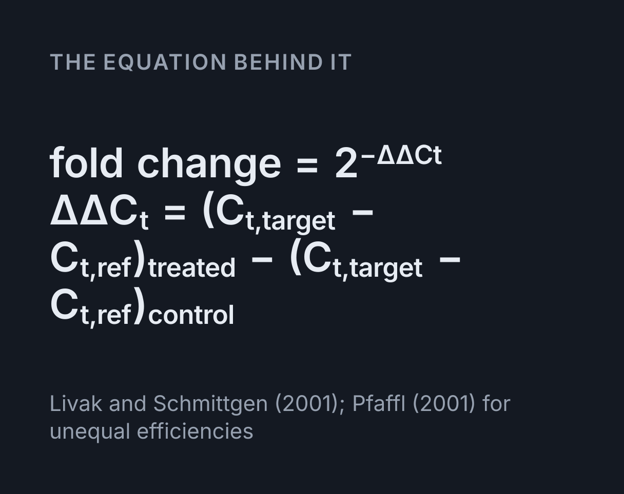
The equation
Livak and Schmittgen (2001); Pfaffl (2001) for unequal efficiencies
What is the delta-delta Ct (ΔΔCt) method?
The delta-delta Ct method, also called the comparative Ct method, turns the threshold cycles from
a qPCR run into a fold change in gene expression. Subtract the reference gene’s Ct from the
target gene’s Ct in each sample to get ΔCt, subtract the control’s ΔCt from the treated
sample’s to get ΔΔCt, and raise 2 to minus that: fold change = 2^−ΔΔCt, where
ΔΔCt = (Ct target − Ct reference)treated − (Ct target − Ct reference)control.
Livak and Schmittgen set it out in 2001, and it remains the usual way to report relative
expression from real-time RT-PCR.
It works because a Ct is a logarithm. At 100% efficiency the product doubles every cycle, so a well that starts with twice the template reaches the threshold one cycle sooner. The difference between two Cts is then the base-2 logarithm of the ratio of their starting quantities, and raising 2 to it turns it back into the ratio. The minus sign is there because more template means a lower Ct: a ΔΔCt of −3 is a rise of 2³ = 8 times. The reference gene cancels differences in how much material went into each well, and the control sample sets the baseline that the treated sample is compared with.
What a Ct value tells you
A Ct value, the threshold cycle, is the fractional cycle at which a well’s fluorescence first crosses a threshold set above the background. The more template a well starts with, the sooner it crosses. At 100% efficiency each cycle earlier is twice as much template, and a tenfold difference is log₂ 10 = 3.32 cycles. The MIQE guidelines (Bustin and colleagues, 2009) call the same number the quantification cycle, Cq, and some instruments call it the crossing point.
A single Ct is not a quantity. It depends on the threshold, the dye, the instrument and the assay, so equal Cts in two different assays need not mean equal amounts of template. What carries over is the difference between two Cts of the same gene measured the same way, which is why the method compares wells rather than reading any one of them. It is the same doubling arithmetic as a growing culture, which the cell doubling time calculator runs the other way, from two counts to a doubling time.
Reading a qPCR amplification curve
An amplification curve has three stretches. At first the product is too scarce to show above the background, so the curve lies flat. Then comes the exponential phase, where the product grows by the same factor every cycle. On a log fluorescence axis this stretch is a straight line whose gradient is set by the efficiency. Finally primers, nucleotides and enzyme run short, growth slows, and the curve levels off at a plateau.
The plateau says nothing about how much template a well started with. Wells a hundredfold apart reach much the same height, which is why end-point PCR is not quantitative. Quantification uses the exponential phase instead, so the threshold goes there: on the straight part of the log plot, clear of the background noise and well below the plateau, at one height for every well of a gene. Turn on the log fluorescence axis to see the straight stretch the threshold should cross.
Using the simulator
There are two ways in. Ct values from a run takes the four Cts an instrument reported: the target and the reference gene in a control sample and in a treated sample. Enter the mean Ct of the technical replicates for each. The curves are drawn to cross the threshold at those cycles, and the readouts give both ΔCts, ΔΔCt, 2^−ΔΔCt and the Pfaffl ratio. Starting copies and a true change sets the biology instead: how many copies of each gene the control well holds, how much the target really changes, and how much cDNA went into the treated well. The Cts then follow, and you can see whether the method finds the change you set.
Play runs the reaction cycle by cycle, with a dot for each cycle’s reading, and marks each Ct as its curve crosses the dashed threshold. Colour is the gene and the dashes are the sample: the control is dashed and the treated sample solid. In the copies mode you can drag the threshold line, or select the scene and use the arrow keys. Under the scene are the four Cts and each gene’s own change between the samples, and the standard-curve plot draws Ct against log input for a tenfold dilution series of the control cDNA, with the treated wells placed on the same lines.
Worked example: an eightfold rise in a half-loaded well
The simulator opens on a control sample with a target Ct of 26.73 and a reference Ct of 20.08, and a treated sample with a target Ct of 24.73 and a reference Ct of 21.08, with both genes at 100% efficiency.
- Control:
ΔCt = 26.73 − 20.08 = 6.65cycles. - Treated:
ΔCt = 24.73 − 21.08 = 3.65cycles. - Between them:
ΔΔCt = 3.65 − 6.65 = −3.00cycles. - Fold change:
2^−ΔΔCt = 2^3 = 8, an eightfold rise in the target.
Gene by gene, the target’s Ct fell by 26.73 − 24.73 = 2.00 cycles, which on its own looks like a
fourfold rise, 2² = 4. The reference’s Ct rose by 1.00 cycle, which says the treated well held
half as much cDNA, 2⁻¹ = 0.5. A fourfold rise from half the material is an eightfold rise per
unit of cDNA, 4 ÷ 0.5 = 8, which is also the Pfaffl ratio the readouts give. Without
the reference gene, the loading difference would have hidden half of the change.
Switch to starting copies and a true change to see where those Cts come from: 1,000 target copies and 100,000 reference copies in the control well, an eightfold rise in the target, and a treated well with half the cDNA. The reference starts with 100 times the target’s copies, so it crosses log₂ 100 = 6.644 cycles sooner, and all four Cts land within 0.005 of a cycle of the opening values.
Why the reference gene is there
Two samples rarely reach their wells with exactly the same amount of RNA. Extraction yields differ, reverse transcription varies and pipettes are not perfect, so a target can look higher in one sample only because more of everything went in. A reference gene, chosen because the treatment does not change it, measures that difference, and subtracting its Ct cancels it. That is the job ΔCt does before ΔΔCt compares the samples.
Common choices are GAPDH, β-actin and 18S rRNA, but no gene is stable under every treatment, so the choice has to be checked for each experiment. The geNorm approach of Vandesompele and colleagues (2002) ranks candidate genes by how steady they are and normalises to the geometric mean of several. Measuring the RNA by its A260 before reverse transcription, as the nucleic acid quantification calculator does, keeps the loading close, but it does not replace the reference gene: A260 counts all the RNA, not the cDNA of interest that reaches each well.
PCR efficiency and the standard curve
PCR efficiency, E, is the fraction of the template copied in each cycle, so the product grows by
1 + E a cycle: 100% doubles it and 90% multiplies it by 1.9. It is measured with a standard
curve, a dilution series run for each assay with Ct plotted against log₁₀ of the input. The points
fall on a straight line of slope −1/log₁₀(1 + E), and turning that round gives
E = 10^(−1/slope) − 1. A slope of −3.322 is 100%, −3.587 is 90% and −3.103 is 110%.
Most labs accept 90 to 110%. A real efficiency cannot pass 100%, since no strand is copied twice in one cycle, so a higher figure points to a fault in the curve: inhibitors in the most concentrated wells, which delay their Cts and flatten the slope, pipetting errors in the dilutions, or primer-dimer signal in the dilute wells. Low efficiency usually traces back to the primers, whose melting temperatures the primer Tm calculator works out, or to a long amplicon. Livak and Schmittgen’s check that 2^−ΔΔCt is safe is to plot ΔCt against log input for both genes: when the efficiencies match the line is flat, and a slope under 0.1 in size is the usual pass mark. The slope of ΔCt readout gives that figure.
When efficiencies differ: the Pfaffl ratio
2^−ΔΔCt counts every cycle as a doubling. When an assay amplifies at less than 100%, each cycle
is less than a doubling, and the method misreads the change. Pfaffl (2001) gave the correction,
which raises each gene’s own amplification factor to its own Ct shift between the samples:
ratio = (1 + E target)^shift target ÷ (1 + E reference)^shift reference, where each
shift is Ct control − Ct treated for that gene, the quantity Pfaffl writes as ΔCP. With both
genes at 100% it is exactly 2^−ΔΔCt.
-
With the opening Cts, set the target efficiency to 90%. The Pfaffl ratio becomes
1.9^2 ÷ 2^−1 = 3.61 × 2 = 7.22, while 2^−ΔΔCt stays at 8, which is 10.8% too high. - In the copies mode, the same 90% target changes the Cts themselves, because the target now takes more cycles to cover the same fourfold rise: 2.160 cycles rather than 2. ΔΔCt becomes −3.160 and 2^−ΔΔCt reads 8.937 against a true change of 8, while the Pfaffl ratio finds 8 exactly.
-
Set both genes to 90% with the opening Cts and the ratio is
1.9^3 = 6.859. With equal efficiencies Pfaffl’s formula reduces to (1 + E)^−ΔΔCt, so the same ΔΔCt of −3 stands for less than an eightfold rise.
Where the threshold sits changes neither answer, as long as both samples of a gene are read at the same height. In the copies mode at 100% efficiency, raising the threshold from 10% to 20% of the plateau makes every Ct 1.170 cycles later and leaves ΔCt, ΔΔCt and the fold change as they were.
Relative or absolute quantification
The ΔΔCt method is relative quantification: it says how many times more target the treated sample holds than the control, not how many copies either one contains. Absolute quantification needs a standard curve of known amounts, such as a plasmid or a synthetic fragment measured by A260 and diluted tenfold, and reads each unknown off that line from its Ct. Digital PCR counts molecules directly instead, by splitting a sample into thousands of partitions and counting the ones that amplify.
The two kinds of reading agree. On the standard-curve plot the treated wells sit at
log₁₀ 4 = 0.602 on the target’s line and log₁₀ 0.5 = −0.301 on the
reference’s, and the gap between them, 0.903, is log₁₀ 8: the same eightfold rise, read off the
lines rather than worked out from the Cts.
What this model leaves out
- Replicates and statistics. Real experiments run technical and biological replicates. Statistics are done on the ΔCt values and converted to a fold change only at the end, which is why error bars on a fold change are not symmetric.
- Noise and the baseline. Measured fluorescence sits on a background that software estimates from the early cycles, often cycles 3 to 15, and subtracts. The curves here start from zero and have no noise.
- Very low copy numbers. With only a few tens of copies or fewer, chance decides how many molecules each replicate receives, so replicate Cts scatter. Here every well holds exactly its expected number of copies.
- What is amplified. A dye such as SYBR Green binds any double-stranded DNA, so primer-dimers and off-target products add signal. A single peak in a melt curve, or a single band of the right size on a gel like those in the gel electrophoresis simulator, confirms one product. Here every curve is the intended product alone.
- Reverse transcription. The cDNA is taken as a faithful copy of the RNA. Real reverse transcriptase converts different transcripts with different efficiencies, which cancels only when it is the same in both samples.
- Efficiency that changes from sample to sample. Each assay has one efficiency here, shared by the control and the treated sample. An inhibitor carried over from one extraction lowers that sample’s efficiency alone, and neither method corrects for it.
- The shape of the curve. The curves follow the logistic sigmoid that Rutledge (2004) fitted to real runs, with one plateau of 10¹² copies for every well. Real plateaus vary from well to well, which does not move a Ct read in the exponential phase.
Common mistakes
- Subtracting the wrong way round. ΔCt is target minus reference and ΔΔCt is treated minus control. Reversing either one flips the sign and turns a rise into a fall.
- Dropping the minus sign. 2^ΔΔCt in place of 2^−ΔΔCt turns the opening eightfold rise into a fall to 0.125.
- Averaging fold changes. Average the ΔCt or ΔΔCt values, then convert. Replicates at ΔΔCt values of −2 and −4 average to −3, an eightfold rise, while their fold changes, 4 and 16, average to 10.
- Assuming 100% efficiency without checking. With the target at 90% and the reference at 100%, the opening Cts give 8 by 2^−ΔΔCt and 7.22 by the Pfaffl ratio. A standard curve for each assay settles which figure to trust.
- Trusting a reference gene the treatment changes. If the treatment doubles the reference gene, every fold change comes out at half its true size.
- Comparing Cts read at different thresholds. A Ct only means something against other Cts of the same gene read at the same threshold. Runs on different plates need a shared calibrator sample to line them up.
Model and assumptions
- Method
- Exact expression, no time stepping
- Repeatability
- Deterministic. The same link gives the same numbers on any machine.
What it assumes
- Each well’s fluorescence follows the logistic curve Rutledge (2004) fitted to real runs: it grows by the factor 1 + E each cycle while product is scarce, then levels off at a plateau of 10¹² copies shared by every well.
- The Ct is where that curve crosses the threshold, solved exactly, so two wells of one gene differ in Ct by exactly the logarithm, to base 1 + E, of the ratio of their starting copies.
- Each gene’s efficiency is the same in the control and the treated sample, so a gene’s two curves are parallel and ΔΔCt does not depend on where the threshold is set.
- The reference gene changes only with how much cDNA went into the well, and when the wells are set from copies the treated well holds the control’s cDNA times the loading set.
- Measured Cts are drawn by working each well’s starting copies back from its Ct at a threshold of 10 percent of the plateau, which places the curves on the scene and changes no result.
- A well that does not reach the threshold within the 40 cycles has no Ct, as instrument software reports it undetermined, and every comparison that needs it is left blank.
- Fluorescence has no noise, baseline drift or primer-dimer signal, every well holds exactly its expected number of copies, and reverse transcription converts each transcript equally well in both samples.
Where it stops holding. Very low template, where Poisson sampling of the few molecules in each well scatters replicate Cts, and samples whose efficiency is lowered by an inhibitor carried over from extraction, which neither 2^−ΔΔCt nor the Pfaffl ratio corrects.
Numerical accuracy
No method error to report: the result is a closed-form expression evaluated directly, with no time stepping to accumulate error. What remains is double-precision rounding, of order one part in 10^16 per operation.
Common questions
How do you calculate fold change from Ct values with the ΔΔCt method?
Subtract the reference gene’s Ct from the target’s in each sample to get ΔCt, subtract the control’s ΔCt from the treated sample’s to get ΔΔCt, then take 2^−ΔΔCt. With a control at target 27.50 and reference 19.10, and a treated sample at target 25.90 and reference 19.30, the ΔCts are 8.40 and 6.60, ΔΔCt is 6.60 − 8.40 = −1.80, and the fold change is 2^1.80 = 3.48, a 3.48-fold rise. Use the mean Ct of the technical replicates for each well.
What does a negative ΔΔCt mean?
That the target is more abundant in the treated sample than in the control once both are normalised to the reference gene: the treated sample reached the threshold sooner. A ΔΔCt of −1 is a doubling and −3 an eightfold rise. A positive ΔΔCt is a fall: 1.5 gives 2^−1.5 = 0.354, a little over a third of the control’s level. At 100% efficiency, −ΔΔCt is the log₂ fold change, which is the figure to plot or average.
What is a Ct value in qPCR?
The threshold cycle: the fractional cycle at which a well’s fluorescence crosses a threshold set in the exponential phase of amplification. The more template a well starts with, the sooner it crosses, so a lower Ct means more target. At 100% efficiency each cycle earlier is twice as much template, and 3.32 cycles is ten times as much. Cts are compared rather than read alone, because each one depends on the threshold, the dye and the instrument. The MIQE guidelines call it the quantification cycle, Cq.
What is a good PCR efficiency, and how is it calculated?
Run a tenfold dilution series, plot Ct against log₁₀ of the input and take the slope: E = 10^(−1/slope) − 1. A slope of −3.322 is 100% efficiency, a doubling every cycle, while −3.587 is 90% and −3.103 is 110%. Most labs accept 90 to 110%. A true efficiency cannot be above 100%, so a higher figure usually means inhibition in the concentrated wells, a pipetting error in the dilutions or primer-dimers in the dilute ones.
When should I use the Pfaffl method instead of 2^−ΔΔCt?
When the target and reference assays do not both amplify at close to 100% efficiency. The Pfaffl ratio raises each gene’s amplification factor, 1 + E, to its own Ct shift, control minus treated, and divides the target’s by the reference’s. With Cts of 26.73 and 20.08 in the control and 24.73 and 21.08 in the treated sample, 2^−ΔΔCt gives 8. With the target at 90% efficiency the Pfaffl ratio is 1.9² ÷ 2⁻¹ = 7.22, so 2^−ΔΔCt is 10.8% too high.
Should I average fold changes or ΔCt values?
Average the ΔCt or ΔΔCt values and convert to a fold change at the end. Fold changes are exponential, so a plain average of them is pulled up by the largest: replicates with ΔΔCt values of −2 and −4 average to −3, an eightfold rise, but their fold changes of 4 and 16 average to 10. Error bars work the same way, worked out on the ΔCt scale and uneven once converted.