Radioactive Decay Simulator

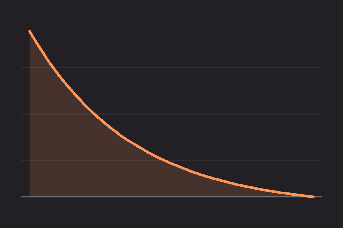
The formula is an average, not a schedule

N = N₀e^(−λt) is the single most recognisable equation in this topic, and it describes something subtly different from what actually happens. Decay is random: each nucleus has a fixed probability of going in any given interval, and nothing coordinates them. The exponential is what you get by averaging that randomness over a large number of nuclei.

With 5000 dots above, the count sits so close to the curve that the distinction looks academic. Drop to 20 and it stops looking academic: the count staircases downwards, and pressing Fresh sample twice with identical settings gives two different answers. Neither run is wrong. The formula was never promising either of them.

Why the scatter shrinks as the sample grows

The number decaying in a fixed window is a count of independent random events, so its spread goes as the square root of the count while the count itself goes up linearly. The relative scatter therefore falls as 1/√N. At 100 nuclei that is about 10 percent; at 10,000 it is about 1 percent.

This is why a smoke detector containing an almost unimaginable number of americium nuclei has an utterly predictable activity, and why counting a weak laboratory source for ten seconds gives a figure you should not quote to three significant figures. The Difference readout above is this effect, live.

Half-life, mean lifetime, and which one to use

The half-life is the time by which half the sample has gone. The decay constant is λ = ln 2 / t½, and the mean lifetime of a single nucleus is 1/λ, which is about 1.44 half-lives. Those last two are not the same number and the difference is not rounding.

The half-life is a median: half the nuclei have gone by then. The mean lifetime is an average, and it is longer because a few nuclei survive an extremely long time and pull the average up. For a 6 second half-life the average nucleus lasts 8.66 seconds.

Nuclei do not age

A nucleus that has already survived ten half-lives is exactly as likely to decay in the next second as one created a moment ago. There is no internal clock counting down and no wear. This memorylessness is the reason the curve is exponential and not some other decreasing shape, and it is the property that makes the whole thing so unlike anything in ordinary experience, where old things are more likely to fail than new ones.

It also means “half-life” says nothing about any individual nucleus. It is a statement about populations only. Asking when a particular atom will decay has no answer beyond a probability distribution.

Activity is what a detector actually measures

You cannot see the number of surviving nuclei. What an instrument counts is decays per second, the activity A = λN, measured in becquerels. Because it is proportional to N, it falls with the same half-life, so a plot of activity against time has the same shape as the count.

The second graph above is deliberately jagged. Each point is the number of decays in a one second window, and that is a random count, so it fluctuates even when the underlying rate is changing smoothly. Real counting experiments average over longer windows to suppress this, trading responsiveness for precision.

What this model leaves out

One decay path, one product, and a product that is stable. Real chains are longer: uranium-238 passes through fourteen steps before it reaches lead. Where a daughter is itself radioactive the population of the intermediate rises and then falls, which needs a coupled set of equations rather than one.

There is also no detector here. A real measurement misses most decays, because the counter only intercepts part of the solid angle and only registers some of what reaches it, so measured counts sit well below the true activity. And the background never goes away, which is why a real experiment measures it separately and subtracts it.

Common mistakes

• Treating the formula as exact for a small sample. It is an average. With tens of nuclei the actual count deviates from it by a large fraction.
• Using the half-life as the mean lifetime. They differ by a factor of 1/ln 2, about 1.44.
• Thinking decay speeds up as a sample ages. The rate per surviving nucleus is constant. The total rate falls only because fewer nuclei remain.
• Assuming the sample is gone after a few half-lives. After ten it is down to about a thousandth, not to zero. Exponentials do not reach zero.
• Using λ dt as the decay probability over a long interval. Over one half-life that gives 0.693 where the true figure is 0.5, an overestimate of 39 percent. The exact form is 1 − e^(−λt).
• Quoting a measured activity as the true activity. A detector sees a fraction of the decays, and background adds to whatever it does see.