Pharmacokinetics Dosing Simulator
A pharmacokinetics simulator for repeated IV bolus, infusion or oral doses. Watch drug accumulation reach steady state against a therapeutic window.
Simulator
Use the left and right arrow keys to step from dose to dose, and Home and End to jump to either end. Space plays and pauses.
Concentration against time over 72 h: 12 IV bolus doses of 250 mg every 6 h. The levels climb towards a steady state that runs from 10.48 to 17.62 mg/L around an average of 13.74 mg/L, inside the window, which is shaded from 10 to 20 mg/L. At 0 h the concentration is 7.143 mg/L.
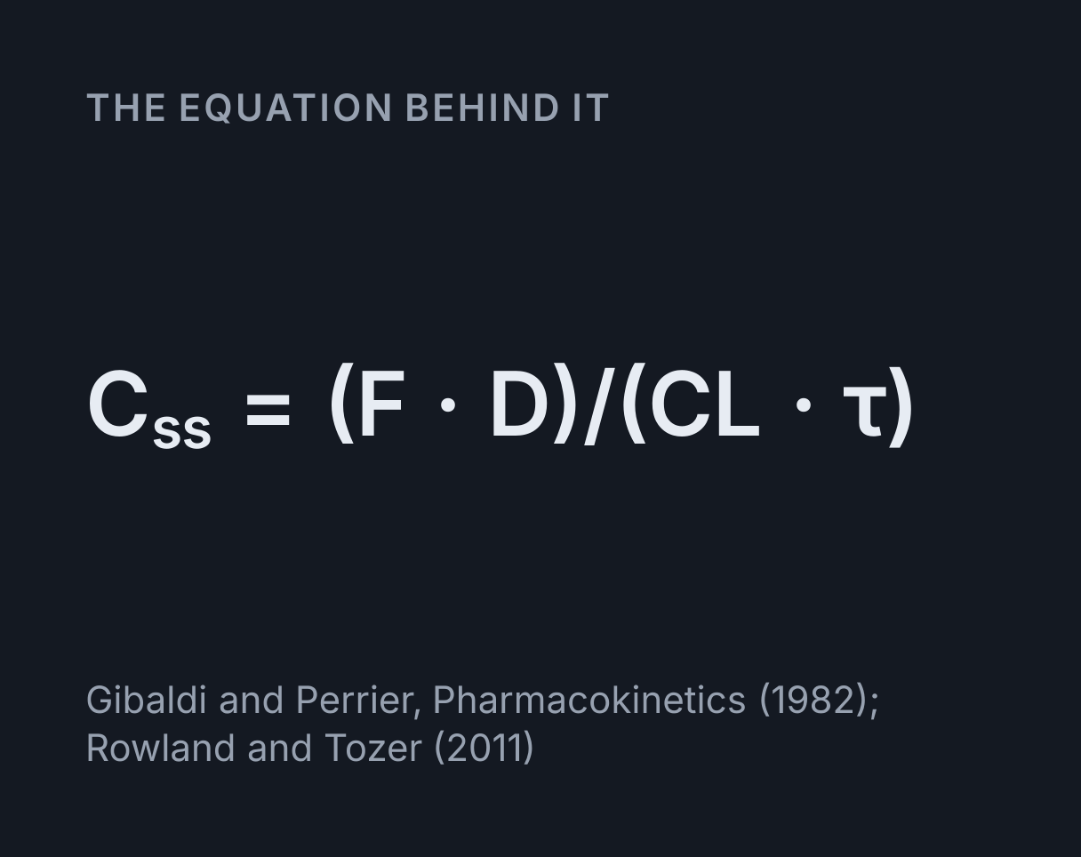
- Average at steady state Css = F × D / (CL × τ) = 1 × 250 / (3.033 × 6): the dose rate that reaches the blood over the clearance. The route moves the peak and the trough around it, not the average.
- 13.74 mg/L
- Peak at steady state (D / V) × R = 7.143 × 2.467: the level one dose gives, times the accumulation factor, straight after each dose.
- 17.62 mg/L
- Trough at steady state Cmax × e^(−kτ) = 17.62 × 0.5946: the peak after one interval of decay, just before the next dose.
- 10.48 mg/L
- Concentration now What is left of the first dose given by t = 0 h, added together. Each dose decays on its own, whatever else is in the body.
- 7.143 mg/L
- Accumulation factor R = 1 / (1 − e^(−kτ)) = 1 / (1 − 0.5946). Each dose finds 59.5 percent of the one before still in the body, and for an IV dose the steady-state peak and trough are R times the first ones.
- 2.467
- Time to steady state Four to five half-lives, by which the levels are 93.75 and 96.9 percent of the way to steady state. 90 percent takes ln 10 / k = 26.58 h. The dose and the interval do not change it.
- 32 to 40 h
- Loading dose D × R = 250 × 2.467. Given as the first dose it puts every level at steady state from the start.
- 616.7 mg
- Doses that fit the window Every maintenance dose in this range keeps the steady-state trough at or above 10 mg/L and the peak at or below 20 mg/L at this interval, because every level is proportional to the dose.
- 238.6 to 283.8 mg
- AUC per interval F × D / CL: the area under one interval at steady state, which equals the whole area under a single dose. Divided by τ it is the average.
- 82.44 mg·h/L
- Clearance CL = k × V = 0.08664 × 35: the volume of plasma cleared of drug each hour.
- 3.033 L/h
- Elimination rate constant k = ln 2 / t½ = 0.6931 / 8: the fraction of the drug in the body removed per hour, at any instant.
- 0.08664 h⁻¹
A teaching model, not a dosing tool. Real doses are set from measured levels and clinical judgement.
- Steady state
- After the first dose
- Steady-state average
- Window limits
Citing this tool
Last updated . Add the date you accessed it as well, which a citation of a page that can change asks for. If a specific result matters, cite the permalink from the tool’s share row instead of this page: it reproduces the exact parameters.
The equation
Gibaldi and Perrier, Pharmacokinetics (1982); Rowland and Tozer (2011)
What is a pharmacokinetics simulator?
A pharmacokinetics simulator predicts how the concentration of a drug in the blood rises and
falls over a course of doses, from the dose, the dosing interval and how quickly the body
removes the drug. This one uses the one-compartment model with first-order elimination, which
sits behind most dosing calculations. Each dose adds to whatever is left of the doses before
it, so the levels climb until the drug eliminated in each interval matches one dose. At that
steady state the average concentration is Css = F × D / (CL × τ): the part of
the dose that reaches the blood, divided by the clearance and the interval.
Here k = ln 2 / t½ is the elimination rate constant and CL = kV is the clearance, the volume of plasma cleared of drug each hour. The doses can go in as an IV bolus, as an IV infusion of set length or by mouth with first-order absorption, and the curve is drawn against a therapeutic window: the range between the lowest concentration that works and the level above which toxic effects become likely. This is a teaching model, not a dosing tool. Real patients are dosed from measured levels and clinical judgement.
Using the simulator
Choose the route, then set the maintenance dose, the dosing interval τ, the elimination half-life and the volume of distribution. An infusion also takes its infusion time, and an oral dose its absorption rate constant ka and bioavailability F. Play runs the regimen and the scrubber moves through it by hand. With the graph focused, the left and right arrow keys step from one dose to the next.
The main graph shows the concentration over the whole run, with a mark under each dose and the stretch from four to five half-lives shaded. The grey dashed line is the steady-state average. The graph below overlays one dosing interval at steady state on the interval after the first dose, so the gap between the two curves is the accumulation. The readouts give the steady-state levels, the accumulation factor, the time to steady state, a loading dose and the doses that fit the window.
How repeated doses build up to steady state
With first-order elimination every dose decays on its own, whatever else is in the body, so
the concentration at any moment is the sum of what remains of every dose so far. This is
superposition, and it is how every point here is computed. After an IV bolus a fraction
r = e^(−kτ) of each dose is still there when the next arrives,
so just after the nth dose the level is C0(1 + r + r² + … + r^(n−1)), where C0 = D/V is the
level one dose gives. The geometric series adds up to a steady-state peak of
Cmax = C0 / (1 − e^(−kτ)), and the trough is that peak times r.
The factor 1/(1 − e^(−kτ)) is the accumulation factor R. It depends only on the interval measured in half-lives. Dose once every half-life and r = 0.5, so R = 2: the steady-state peak is twice the first peak, and the trough equals the first peak. Dose more often and R grows; dose rarely and it falls towards 1, because each dose has almost gone before the next.
How fast the plateau is approached depends on the half-life alone. After dosing for a time t, the trough before the next dose has covered 1 − e^(−kt) of the way to steady state: half after one half-life, 90 percent after 3.32, 93.75 percent after four and 96.9 percent after five. That is the rule that steady state takes four to five half-lives. A bigger dose raises the plateau and a shorter interval smooths it, but neither gets there sooner.
Worked example: 250 mg every 6 hours with an 8 hour half-life
The simulator opens on an IV bolus of 250 mg every 6 h, with a half-life of 8 h, a volume of distribution of 35 L and a window of 10 to 20 mg/L. Those are close to theophylline in a non-smoking adult, with the British National Formulary’s 10 to 20 mg/L range, though theophylline is not given as a bolus.
-
Elimination:
k = ln 2 / 8 = 0.086643 h⁻¹andCL = 0.086643 × 35 = 3.0325 L/h. -
The first dose gives
C0 = 250 / 35 = 7.143 mg/L, below the 10 mg/L lower limit. -
Each interval is 0.75 half-lives, so
r = e^(−0.086643 × 6) = 0.5946of each dose is left when the next is given. - Accumulation factor:
R = 1 / (1 − 0.5946) = 2.467. -
Steady-state peak:
Cmax = 7.143 × 2.467 = 17.62 mg/L. Trough:Cmin = 17.62 × 0.5946 = 10.48 mg/L. Both sit inside the window. -
Average:
Css = 250 / (3.0325 × 6) = 13.74 mg/L, and the area under one interval isAUC = 13.74 × 6 = 82.44 mg·h/L, the same as the area under one whole dose, D/CL. -
Time to steady state: 90 percent after
3.322 × 8 = 26.58 h, and four to five half-lives is 32 to 40 h. -
Loading dose:
LD = 17.62 × 35 = 616.7 mg, the steady-state peak times the volume, which is the same as D × R. -
Doses that fit: anything from
250 × 10 / 10.477 = 238.6 mgto250 × 20 / 17.619 = 283.8 mg, worked from the unrounded trough and peak, keeps the steady state inside 10 to 20 mg/L at this interval.
Play the run and the early doses fall short: the first peak is only 7.143 mg/L, and every trough dips below 10 mg/L until the one just before the seventh dose, at 36 h, which reaches 10.01 mg/L. The fifth trough, at 30 h, is 9.698 mg/L. That day and a half spent partly below the window is what a loading dose is for.
Loading doses
A loading dose is a larger first dose that puts the levels where the steady state will be, so
the drug works from the first dose. For repeated IV boluses the dose that does it exactly is
the maintenance dose times the accumulation factor, LD = D × R. Tick Start with a
loading dose and the curve is at steady state from the first dose: 616.7 mg and then 250 mg every 6 h
peak at 17.62 mg/L every time, and the two curves on the lower graph lie on top of each other.
The other common form is LD = Ctarget × V / F for any target concentration.
Aiming at the average, 13.74 mg/L, gives 13.74 × 35 = 480.9 mg, which starts the
levels mid-window rather than at the peak. For an infusion, D × R run in over the usual
infusion time reaches the steady-state peak at the end of the first infusion, and
from then on the curve is the steady state exactly. For an oral dose it gives very nearly the
steady state once the first dose is absorbed, and less before that, while the level climbs
from nothing.
Fitting the regimen to the therapeutic window
Two things have to fit. The average sets where the levels sit, and it depends only on the dose
rate D/τ, the clearance and, by mouth, F. The swing sets whether they fit, and for an IV bolus
the peak-to-trough ratio is Cmax / Cmin = e^(kτ), which depends only on the
interval in half-lives. The window has a ratio of its own, 20/10 = 2 here, so the longest
interval that can fit is τmax = ln(20 / 10) / k = 8 h, exactly one half-life, and
the only dose that fits at that interval is V × (20 − 10) = 350 mg, which runs
from exactly 10 to exactly 20 mg/L.
At 6 h the swing is e^(0.086643 × 6) = 1.682, narrower than the window, which is
why a range of doses fits. Lengthen the interval to 12 h and the swing becomes 2.83: no dose
fits, and the readout says none, because a dose large enough to hold the trough at 10 mg/L
takes the peak past 20 mg/L. Doubling the dose cannot help, since it doubles the peak and the
trough alike. That is why drugs with a narrow window and a short half-life are given often, by
continuous infusion or as modified-release tablets.
Infusions and oral doses
An infusion delivers each dose at a constant rate over its infusion time T. The level rises
while it runs and falls after it stops, so the peak comes at the end of each infusion:
Cmax = D (1 − e^(−kT)) / (CL T (1 − e^(−kτ))), with the trough e^(−k(τ − T))
times that, the form Sawchuk and Zaske used for gentamicin in 1976. The opening 250 mg run in
over 1 h every 6 h peaks at 16.88 mg/L and falls to 10.94 mg/L. Stretch the infusion to the
whole interval and it becomes a continuous infusion: the swing vanishes and the level settles
at the average, 13.74 mg/L.
An oral dose has to be absorbed first. With first-order absorption at rate constant ka, a
single dose follows the Bateman function,
C = F D ka (e^(−kt) − e^(−ka t)) / (V (ka − k)). At steady state the peak comes at
t′max = ln[ka(1 − e^(−kτ)) / (k(1 − e^(−kaτ)))] / (ka − k) after each dose, as
Gibaldi and Perrier give it. Switch the opening regimen to Oral, with ka = 1 h⁻¹ and F = 1,
and the peak falls to 15.22 mg/L, 1.692 h after each dose, while
the trough rises to 11.45 mg/L. The average stays at 13.74 mg/L, because absorption changes
when the drug arrives and not how much of it does. F does change it: at F = 0.5 every level
halves, and the average is 6.87 mg/L.
When absorption is slower than elimination, with ka below k, the slow fall after each peak is set by absorption rather than elimination. This is called flip-flop kinetics, and it also slows the approach to steady state, which then takes roughly four to five absorption half-lives. The simulator says so when it happens. Many modified-release tablets behave this way by design.
Half-life, clearance and volume
The three are tied by t½ = 0.693 V / CL, and each controls something different.
Clearance sets the average for a given dose rate. The volume sets how far a single dose lifts
the level, D/V, and so the size of the swing. The half-life follows from the two and sets both
the time to steady state and how far the levels fall between doses. Double the volume at the
same clearance, which here means doubling both the volume and the half-life, and the average
stays where it was while the swing narrows and steady state takes twice as long.
Clearance is where the patient comes in. A drug cleared by the kidneys, such as gentamicin or digoxin, has a clearance that falls with kidney function, which is why dosing guides lean on the creatinine clearance from the eGFR and creatinine clearance calculator, and some cytotoxic drugs are dosed by body surface area instead of weight. Digoxin also shows why the upper limit matters: above its narrow range it slows conduction through the heart, causing the kind of blocked beats the ECG rhythm and heart block simulator draws. The fall between doses is the same first-order decay as a radioactive sample’s, and the half-life calculator gives the fraction left after any time.
What this model leaves out
- A distribution phase. Many drugs fall fast at first as they spread into the tissues, then more slowly as they are eliminated, which needs two or more compartments. Digoxin levels mean little until distribution is over, at least six hours after a dose.
- Saturable elimination. Phenytoin, alcohol and high-dose aspirin saturate the enzymes that remove them at the levels they are used at, so the half-life lengthens as the level rises and a small rise in dose can cause a large rise in level.
- A changing patient. Kidney and liver function, body weight and interacting drugs change clearance and volume over days, and carbamazepine speeds up its own clearance over the first weeks of treatment.
- Protein binding. The model follows the total concentration. Only the unbound drug acts, and the bound fraction changes with albumin and disease.
- Real absorption. Oral doses can start after a lag, be slowed by food, absorb in stages or be partly destroyed by first-pass metabolism, which F stands in for.
- Missed and late doses. Every dose here is the same size and on time. A missed or doubled dose changes the levels for several half-lives afterwards.
- Variation between people. The same regimen gives different levels in different patients, several-fold for drugs such as theophylline, which is why narrow-window drugs are measured rather than predicted.
Common mistakes
- Expecting a bigger dose to reach steady state sooner. The time depends only on the half-life. A bigger maintenance dose raises the plateau; only a loading dose gets there faster.
- Using the half-life where k belongs. The exponent is kτ with k = ln 2 / t½. Writing e^(−8 × 6) instead of e^(−0.086643 × 6) turns a 59 percent carry-over into almost none.
- Leaving F out for an oral dose. The average is F × D / (CL × τ), so with F = 0.5 it is half the IV figure.
- Checking only the average against the window. The average can sit mid-window while the peak and trough fall outside it. Lengthen the interval at the same daily dose and the average does not move, but the swing grows.
- Treating the accumulation factor as a constant. R is 2 only when the interval equals the half-life. It is 2.467 at the opening 6 h interval and 1.143 at three half-lives.
- Mixing units. Milligrams over litres give mg/L, which is the same as µg/mL. A dose in micrograms or a half-life in minutes left unconverted shifts the answer by a factor of a thousand or sixty.
Model and assumptions
- Method
- Exact expression, no time stepping
- Repeatability
- Deterministic. The same link gives the same numbers on any machine.
What it assumes
- The body is one well-mixed compartment of fixed volume, so each dose spreads through it at once and there is no separate distribution phase.
- Elimination is first order: the rate of removal is the clearance times the concentration, so the half-life is the same at every level and every dose.
- An IV bolus enters all at once, an infusion at a constant rate over its set time, and an oral dose is absorbed at a rate proportional to what is left to absorb, with no lag time.
- Every dose is the same size and on time, and the half-life, volume, absorption rate and bioavailability stay fixed over the whole run. The loading dose, when it is on, replaces only the first dose and is given the same way.
- Every concentration is the sum of each dose’s own exact curve, and the steady-state peak, trough and average are those sums over every dose ever given, in closed form, so nothing is stepped.
- Time to steady state is quoted as four to five elimination half-lives, which is exact for IV doses and holds for oral doses only when absorption is much faster than elimination.
Where it stops holding. For drugs with a slow distribution phase, such as digoxin, whose levels in the first hours after a dose a single compartment does not describe; and for drugs whose elimination saturates at the levels they are used at, such as phenytoin, alcohol and high-dose aspirin, where removal follows Michaelis-Menten kinetics rather than a fixed half-life. The Enzyme Kinetics Simulator is the right tool there.
Numerical accuracy
No method error to report: the result is a closed-form expression evaluated directly, with no time stepping to accumulate error. What remains is double-precision rounding, of order one part in 10^16 per operation.
Common questions
How do you calculate the steady-state concentration?
The average concentration at steady state is Css = F × D / (CL × τ): the part of each dose that reaches the blood, divided by the clearance and the dosing interval. For 250 mg every 6 h with a clearance of 3.0325 L/h it is 250 / (3.0325 × 6) = 13.74 mg/L. The peak and trough around that average depend on the route and on the interval measured in half-lives. For an IV bolus the steady-state peak is (D/V) / (1 − e^(−kτ)) and the trough is that peak times e^(−kτ), here 17.62 and 10.48 mg/L.
How many half-lives does it take to reach steady state?
About four to five. After four half-lives of regular dosing the levels are 93.75 percent of the way to steady state and after five 96.9 percent, while 90 percent takes 3.32 half-lives. With an 8 h half-life that is 32 to 40 h, whatever the dose or the interval, because the approach depends only on how fast the drug is eliminated. A larger dose raises the plateau without reaching it sooner, which is what a loading dose is for. When an oral drug is absorbed more slowly than it is eliminated, absorption sets the pace instead.
How do you calculate a loading dose?
Multiply the target concentration by the volume of distribution and divide by the bioavailability: LD = Ctarget × V / F. To start a regimen of IV boluses at its steady-state peak, the target is that peak, and the loading dose works out as the maintenance dose times the accumulation factor, D / (1 − e^(−kτ)). For 250 mg every 6 h with an 8 h half-life that is 250 × 2.4667 = 616.7 mg, given once, followed by the usual 250 mg every 6 h.
What is the accumulation factor?
R = 1 / (1 − e^(−kτ)), the factor by which repeated doses build up over a single dose. For an IV bolus it is exactly the steady-state peak divided by the first peak, and the steady-state trough divided by the first trough. It depends only on the dosing interval measured in half-lives: 2 when the interval equals the half-life, 2.467 at three quarters of a half-life and 1.143 at three half-lives, when little of each dose is left by the time of the next.
Why does a drug accumulate with repeated doses?
Because each dose arrives before the last has gone. With first-order elimination a fixed fraction of the drug, e^(−kτ), is still in the body after each interval: 0.5946 when doses come every 6 h and the half-life is 8 h. The level climbs until the amount eliminated over one interval equals one dose, which is the steady state, and it settles there however long the dosing goes on.
What is a therapeutic window?
The range of concentrations between the lowest that has the intended effect and the level above which toxic effects become likely. For theophylline it is usually given as 10 to 20 mg/L. A regimen fits a window only if its peak-to-trough ratio is no larger than the window’s own ratio, so for an IV bolus the dosing interval can be at most ln(Cupper / Clower) / k, which is exactly one half-life for a window of 10 to 20 mg/L. The simulator shows the doses that fit at the interval set, or says that none do.