SIR Epidemic Model Simulator
Run an SIR or SEIR epidemic: set R₀, the infectious period and vaccination to get the peak, the total infected and the herd immunity threshold, 1 − 1/R₀.
Simulator
- Peak infectious The most people infectious at once, from I_max = I₀ + S₀ − (N/R₀)(1 + ln(R₀S₀/N)). It arrives when the susceptible share has fallen to 1/R₀.
- 23,352 people, 23.4%
- Peak on day When the number infectious is largest, read from the run.
- 32.1
- Total infected Everyone infected at some point, from the final size relation ln(s₀/s∞) = R₀(s₀ + i₀ − s∞). A latent period does not change it.
- 89,266 people, 89.3%
- Herd immunity threshold The immune share, 1 − 1/R₀, above which each case infects fewer than one other person on average.
- 60 %
- R on day 0 R₀ times the share still susceptible after vaccination. Above 1 the outbreak grows; below 1 it shrinks from the start.
- 2.5
- Early doubling time ln 2 / r, with r = γ(R − 1). It holds while nearly everyone is still susceptible.
- 2.31 days
- Day
- 0.0
- Infectious now
- 10 people
- R now R₀ × S/N on this day. It falls through 1 at the SIR peak.
- 2.5
- Susceptible (%)
- Infectious (%)
- Recovered (%)
- Threshold 1/R₀ (%)
- New infections per day (% of population)
Citing this tool
Last updated . Add the date you accessed it as well, which a citation of a page that can change asks for. If a specific result matters, cite the permalink from the tool’s share row instead of this page: it reproduces the exact parameters.
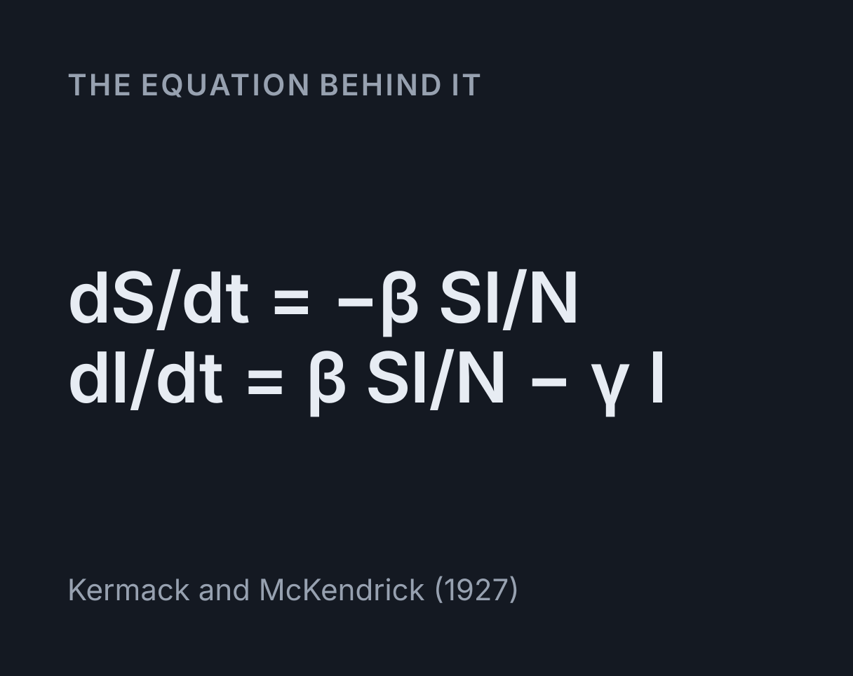
The equation
Kermack and McKendrick (1927)
What the SIR model is
The SIR model splits a population into people who are susceptible (S), infectious (I) and
recovered (R), and moves them between those groups at two rates: new infections at βSI/N per
day and recoveries at γI per day. This simulator solves those equations, or the SEIR version
with a latent stage, for the R₀, infectious period and vaccination you set, and reports the
peak of the outbreak, how many people are infected in the end and the herd immunity
threshold, 1 − 1/R₀.
In plain text the equations are dS/dt = −βSI/N, dI/dt = βSI/N − γI
and dR/dt = γI. N is the population, β the transmission rate per day and
γ = 1/D the recovery rate for a mean infectious period of D days. The basic
reproduction number is R₀ = β/γ: how many people one case infects when everyone
else can catch it. R is often read as removed rather than recovered, since someone who dies of
the infection leaves the chain of transmission in the same way. Kermack and McKendrick
published it in 1927, as the case with constant rates of a more general theory of epidemics.
How to use it
Set R₀ and the infectious period, play the outbreak and watch the squares. Each is a quarter of a percent of the population: blue while susceptible, amber while infected and green once recovered, with the vaccinated drawn as slashed green outlines. The scrubber moves through the days, and the readouts beside the scene give the results for the whole outbreak:
- Peak infectious and Peak on day: the most people infectious at once, and when.
- Total infected: everyone infected at some point, the final size of the epidemic.
- Herd immunity threshold: the immune share,
1 − 1/R₀, above which an outbreak cannot grow. - R on day 0: R₀ times the share still susceptible after vaccination. The outbreak grows only if it is above 1.
- Early doubling time: how quickly the number infected doubles while nearly everyone is still susceptible, the same exponential growth as the cell doubling time calculator works with.
If a problem gives you β and γ rather than R₀, set R₀ to β/γ and the infectious
period to 1/γ days. The rates the equations are using are printed under the
parameters, so you can check the match.
Worked example: R₀ = 2.5 in a town of 100,000
Take the defaults: 100,000 people, 10 of them infectious on day 0, nobody vaccinated, R₀ = 2.5
and an infectious period of 5 days. Then γ = 1/5 = 0.2 per day and
β = R₀γ = 0.5 per day.
- Herd immunity threshold.
1 − 1/2.5 = 0.6, so 60 percent. - Early growth. On day 0, R = 2.5 × 99,990/100,000 = 2.49975, so
r = γ(R − 1) = 0.29995per day and the number infected doubles everyln 2/r = 2.31days at first. - The peak. The number infectious is largest when S has fallen to
N/R₀ = 40,000. The first integral of the equations givesI_max = I₀ + S₀ − (N/R₀)(1 + ln(R₀S₀/N)), here10 + 99,990 − 40,000 × (1 + ln 2.49975), which is 23,352 people, 23.4 percent of the town, on day 32.1. - The total. The final size relation
ln(s₀/s∞) = R₀(s₀ + i₀ − s∞), withs₀ = 0.9999andi₀ = 0.0001, givess∞ = 0.10734: 10,734 people are never infected and 89,266 are, 89.3 percent.
Now switch the model to SEIR with a 5 day latent period, keeping R₀ at 2.5. The doubling time lengthens to 5.96 days, the peak falls to 11,489 and moves to day 80.1, and the total infected is 89,266 again. Go back to SIR and vaccinate 40 percent instead: R on day 0 is 1.5, the peak is 3,788 on day 75.1, and 34,980 people are infected in all, 58.3 percent of the 60,000 who were not vaccinated.
Why the outbreak turns while most people are still susceptible
Rewrite the second equation as dI/dt = γI(R₀S/N − 1). The number infectious
grows while R₀S/N is above 1 and falls once it drops below 1. That product is the
effective reproduction number R, the number of people each case infects now rather than at
the start, and it falls because every infection uses up a susceptible person.
So the peak comes exactly when the susceptible share reaches 1/R₀: 40 percent for
R₀ = 2.5. The dashed line on the first plot marks that level, and in the SIR model the
infectious curve peaks where the susceptible curve crosses it. Read the other way, at that
moment 60 percent of the town can no longer catch it, the 23 percent infectious and the 37
percent recovered, which is the herd immunity threshold: the peak is the moment the
population crosses it.
Herd immunity, and why an epidemic overshoots it
Reaching the threshold stops the growth, not the epidemic. At the peak more people are infectious than at any other moment, and each of them still infects R of the people left, fewer than one but not zero, so infections carry on down the far side of the curve. The final size is therefore well above the threshold. For an outbreak started by a single case in a large population where everyone can catch it, the final size relation and the first integral give:
| R₀ | Herd immunity threshold | Peak infectious | Total infected |
|---|---|---|---|
| 1.5 | 33.3% | 6.3% | 58.3% |
| 2 | 50% | 15.3% | 79.7% |
| 2.5 | 60% | 23.3% | 89.3% |
| 3 | 66.7% | 30.0% | 94.0% |
| 4 | 75% | 40.3% | 98.0% |
| 5 | 80% | 47.8% | 99.3% |
Vaccination works on the same threshold from the other side. Immunise a random share above
1 − 1/R₀ before the first case and R on day 0 is below 1, so the outbreak never
grows. Try it at the defaults. At 59 percent R on day 0 is 1.02, and a slow outbreak peaks at
22 people infectious on day 284 and infects 2,314 in all. At 60 percent R is 0.99975: the
number infectious never rises, though the first ten still pass it on, and 888 people are
infected in all, counting them. At 61 percent the total is 340.
SIR or SEIR: a latent period moves the peak, not the total
The SEIR model adds an exposed class E of people who have been infected but cannot yet infect
anyone: dE/dt = βSI/N − σE, and infectious people now arrive at σE per day, where
1/σ is the mean latent period. R₀ is still β/γ, because everyone who
is exposed goes on to become infectious.
The latent stage slows the start. Wallinga and Lipsitch (2007) showed that when both stages
last exponentially distributed times, as they do here, the early growth rate r and R₀ are
linked by R₀ = (1 + r/σ)(1 + r/γ), against R₀ = 1 + r/γ without one.
At the defaults that takes the growth rate from 0.3 to 0.116 per day. What it does not change
is the total: the final size relation holds unchanged with a latent stage, as Ma and Earn
showed in 2006, so SIR and SEIR with the same R₀ infect the same number of people.
Run the relation the other way and it matters for estimates. The same early growth rate means a larger R₀ with a latent stage than without one, so fitting SIR to an outbreak that has a latent period underestimates R₀. Wearing, Rohani and Keeling (2005) found that ignoring the latent period, or assuming exponentially distributed periods once it is included, always underestimates R₀ from outbreak data.
Reading the two plots
The first plot is the share of the population in each compartment, with the vaccinated as a
flat dashed line when there are any and 1/R₀ dashed in grey. The second is new
infections per day, which is what an epidemic curve of cases by date of infection shows. It
peaks before the number infectious does, because each new infection needs a susceptible
person as well as an infectious one: at the defaults new infections peak on day 28.4 and the
number infectious on day 32.1.
What this model leaves out
Chance. The equations move fractions of a population, so an outbreak with R above 1 always takes off. Real outbreaks start with a few people, and a few people can all recover before passing it on. The radioactive decay simulator shows the same gap between a smooth average and a handful of random events.
Structure. Everyone meets everyone with the same β. Households, schools, ages and travel all make contacts uneven, and with uneven contacts the effect of immunity depends on who has it, so one threshold for a random share no longer tells the whole story.
Time beyond one wave. There are no births, no deaths from other causes and no waning immunity, so the model gives one wave and then stops. Recovery also happens at a constant rate, which makes the infectious period exponentially distributed, the same memoryless shape as radioactive decay in the half-life calculator. Wearing, Rohani and Keeling (2005) call that unrealistic for most infections, whose periods cluster more tightly around their mean.
People reacting. Nobody changes their behaviour, no policy changes during the outbreak, and nothing is seasonal. Those are among the reasons real epidemic curves are rarely the single smooth hump drawn here.
Common mistakes
- Treating R₀ as a fixed property of a pathogen. It is set by how infectious a contact is, how many contacts people have and how long they stay infectious, so the same infection has a different R₀ in a different population.
- Confusing R₀ with R. R₀ assumes everyone else is susceptible. R is R₀ times the share who still are, and it is R that has to be below 1 for cases to fall.
- Expecting the epidemic to stop at the herd immunity threshold. It peaks there and then overshoots it, which is why 89 percent are infected when R₀ = 2.5 and the threshold is 60 percent.
- Using the infectious period as the recovery rate. γ is one over the period: 5 days is 0.2 per day, not 5.
- Assuming the latent period changes the total. It changes when and how high the peak is, not how many are infected in the end.
- Treating the peak in new infections and the peak in people infectious as one day. New infections per day peak first, while the number currently infectious is still rising.
- Taking the curve as a forecast. This is the smooth behaviour of an idealised population. It shows why epidemics rise and fall, not when a real one will.
Model and assumptions
- Method
- Runge-Kutta 4th order
- Fixed step
- 0.01 days
- Repeatability
- Deterministic. The same link gives the same numbers on any machine.
What it assumes
- A closed population of fixed size, with no births, no deaths from other causes and no migration, in which recovery gives lasting immunity, so there is one wave and no endemic state.
- Homogeneous mixing: everyone is equally likely to meet everyone else, so new infections arrive at βSI/N per day with a single β for the whole population.
- People leave the infectious stage, and in SEIR the latent stage, at constant rates, which makes both periods exponentially distributed with the means you set.
- Deterministic and continuous: people are fractions rather than individuals, so an outbreak with R above 1 always takes off and none dies out by chance.
- Vaccination happens once, at random, before the first case, and gives complete and lasting protection.
- The final size, the SIR peak and the early growth rate are closed forms, so they stay exact whatever the step and however long the outbreak runs.
Where it stops holding. Small outbreaks and small populations, where chance decides whether a handful of cases takes off, and populations whose contacts are structured by households, ages or places, where the effect of immunity depends on who has it and one threshold for a random share no longer tells the whole story.
Numerical accuracy
- Estimated error
- 3.2e-8 people in the number of people infectious, about 1.4e-12 of the largest value reached
- How that was obtained
- Running the same problem again at half the step changed the answer by at most 3.0e-8 people over 120 days, the whole outbreak. Richardson extrapolation of that difference gives the figure above.
- Observed order
- 3.83, measured from a second halving rather than assumed
- Conditions
- R₀ 2.5, a 5 day infectious period, 100,000 people with 10 infectious on day 0, SIR, the shipped defaults
The defaults are an easy problem for this step. At the fastest settings the sliders reach, R₀ 20 with a 1 day infectious period, the outbreak peaks within a day and the same step is out by an estimated 1.5 people at a peak of 80,020, about 1.8e-5 of it.
Common questions
What is the SIR model?
A compartment model of an epidemic that splits a population of N people into susceptible (S), infectious (I) and recovered (R), and moves them between the groups at two rates: new infections at βSI/N per day and recoveries at γI per day. Kermack and McKendrick published it in 1927. It assumes a closed population in which everyone is equally likely to meet everyone else, and that recovery gives lasting immunity.
How do you calculate R₀ from β and γ?
Divide β by γ: R₀ = β/γ, which is the transmission rate β multiplied by the mean infectious period D = 1/γ. With β = 0.5 per day and γ = 0.2 per day, R₀ = 2.5, so one case infects 2.5 others on average in a population where everyone can catch it. Adding a latent period, as the SEIR model does, leaves R₀ = β/γ unchanged, because everyone infected goes on to become infectious.
What is the herd immunity threshold, and how is it calculated?
It is the immune share of a population above which each case infects fewer than one other person on average, so an outbreak cannot grow: 1 − 1/R₀. For R₀ = 2.5 it is 60 percent, for R₀ = 4 it is 75 percent and for R₀ = 10 it is 90 percent. In this model, vaccinating more than that share at random before the first case stops the outbreak from taking off.
Why does an epidemic peak while most people are still susceptible?
Because each case now infects R₀ × S/N others, and that falls below 1 once the susceptible share drops under 1/R₀. In the SIR model the number infectious peaks at exactly that moment, with 40 percent still susceptible when R₀ = 2.5. The epidemic then overshoots the herd immunity threshold, because the many people infectious at the peak still pass it on while the curve falls, and about 89 percent are infected in the end.
What is the difference between the SIR and SEIR models?
SEIR adds an exposed class E of people who are infected but not yet infectious, entered at βSI/N per day and left at σE per day, where 1/σ is the mean latent period. The latent stage slows the early growth, lowers the peak and moves it later. With the same R₀ it does not change how many are infected in the end, because the final size relation is unchanged by a latent stage, as Ma and Earn showed in 2006.