Magnetic Field Simulator
Drag bar magnets, wires and coils to see live field lines, iron filings and compass needles, read B anywhere with a probe, and build a Helmholtz coil.
Simulator
Drag anything to move it, or tap to read the field there. Keys: N picks, arrows move, [ and ] turn, F flips.
Show
Magnets
In Earth’s field
Wires
Coils
- Field strength The size of the vector sum of every source’s field at the probe, exact to rounding.
- 1.149 mT
- Direction Anticlockwise from the +x axis, the way a compass needle’s north end would point.
- 0 °
- Bx
- 1.149 mT
- By
- 0 mT
- Against Earth’s field The field here divided by Earth’s horizontal field as set, 20 µT, the part a flat compass feels, whether Earth’s field is switched on or not.
- 57.4 × Earth’s
- Neutral points Where the field is exactly zero in the area the probe can reach, outside the magnets, found by Newton’s method to below 10⁻¹² T: (0, −13.26) cm and (0, 13.26) cm.
- 2
| Source | Distance | Field | Direction |
|---|---|---|---|
| Magnet 1 | 11.7 cm | 973 µT | 53.8° |
| Magnet 2 | 11.7 cm | 973 µT | −53.8° |
| Total | 1.149 mT | 0° |
The fields add as vectors, head to tail as the scene draws them faintly at the probe, so the total is not the sum of the column. Neutral points, where the field is exactly zero in the area the probe can reach, outside the magnets: (0, −13.26) cm and (0, 13.26) cm.
Citing this tool
Last updated . Add the date you accessed it as well, which a citation of a page that can change asks for. If a specific result matters, cite the permalink from the tool’s share row instead of this page: it reproduces the exact parameters.
On the syllabus: AP Physics 2, Unit 12: Magnetism and Electromagnetism.
The equation
Biot and Savart (1820), with Ampère (1823)
What is the magnetic field formula around a straight current-carrying wire?
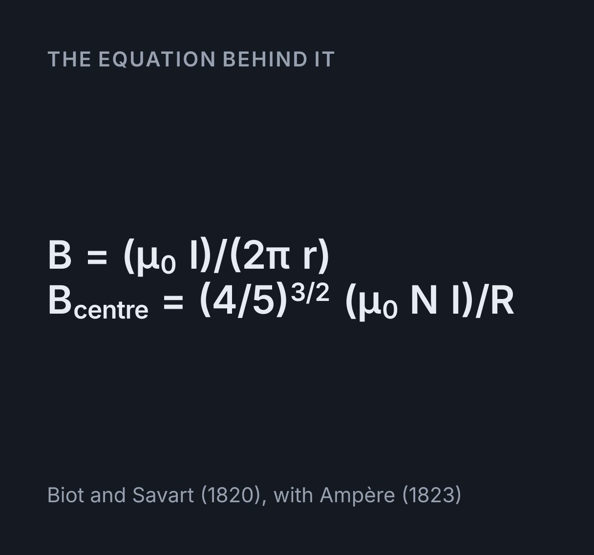
The magnetic field around a long straight wire carrying electric current I is given by the Biot-Savart law: B = (μ0 · I) / (2πr), where B is magnetic flux density in teslas (T), μ0 ≈ 4π × 10−7 T·m/A is the permeability of free space, measured rather than exact since the 2019 SI, I is current in amperes, and r is perpendicular distance in metres.
How to read a magnetic field picture
The scene shows one field three ways, all worked out from the same exact sums. A field line runs along the field everywhere, and its arrows say which way. Outside a magnet the lines leave the north pole and curve round to the south pole; inside it they run from south to north, so every line is a closed loop. Two lines never cross, because the field has only one direction at each point. Each stretch of line is a deeper teal the stronger the field is there, and with Flow on, pulses run along the lines the way the field points, faster where it is stronger.
Iron filings each become a tiny magnet and swing into line with the field, so they show its direction everywhere at once and gather where it is strong. They cannot show which way it points. A compass can: its needle is a magnet free to turn, and its north end, red here, comes to rest pointing along the field. That is why a compass beside a magnet’s north pole points away from it.
Drag a magnet by its body, or turn it by the round handle off its north end, which moves in steps of 15°, or freely with Shift held. Wires and coils move by their symbols, and a coil’s ⊗ sets its radius. Tap anywhere to send the probe there. The scene holds up to 6 objects, and the chips under it switch each view on and off and offer 10 arrangements to begin from. The readouts give the field at the probe in µT, mT or T, its direction anticlockwise from +x and its two components, and the table gives each source’s share.
Bar magnets: why the field loops through the magnet
A uniformly magnetised bar makes exactly the field of a solenoid the same size. That is Ampère’s equivalence: each atom carries a tiny circulating current, neighbouring currents cancel inside the bar, and what is left is a sheet of current round its sides, Br/μ₀ amperes per metre of length, where Br is the magnet’s remanence. So the field runs through the bar from south to north, the way it runs through a coil, and loops back round outside.
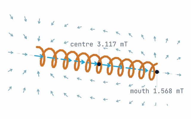
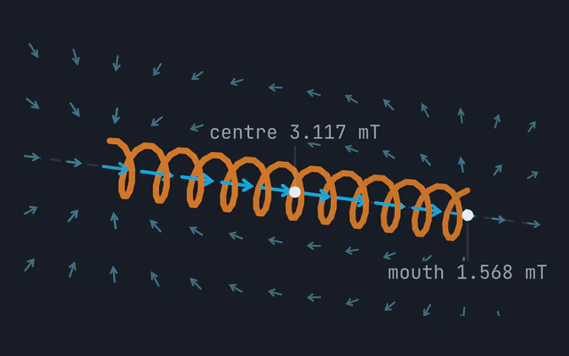
For a 5 cm by 1.2 cm ferrite bar, with Br about 0.39 T, the field is 0.379 T at its centre and 0.194 T at the middle of each pole face, 51 percent of it. That is the same halving the solenoid magnetic field simulator shows at a coil’s mouth, for the same reason: at the face, all of the bar lies on one side. A centimetre beyond the face the field has fallen to 26.8 mT. The same bar in NdFeB of grade N42, about 1.3 T, gives 0.645 T at its face.
The bar’s dipole moment is m = Br πa²L/μ₀, 1.755 A m² for this one. Far away its field
is a point dipole’s of that moment, but only far away: the two agree to within 2 percent at five
lengths from the centre and to within 1 percent past about seven.
Wires and the right-hand grip rule
The field of a long straight wire runs in circles round it, B = μ₀I/(2πr). Point your
right thumb along the current and your fingers curl the way the field goes: anticlockwise here for
a current coming out of the page, drawn ⊙. A current of 10 A gives 40 µT at 5 cm, twice Earth’s
horizontal field in London, and 20 µT at 10 cm, since twice as far away the field is half as strong.
Two wires with currents the same way pull on each other, and with opposite currents they push
apart. With 10 A in each, 10 cm apart, the force is μ₀I₁I₂/(2πd), 0.2 mN on every metre
of wire. Between same-way currents the fields cancel, at a neutral point midway; between opposite
ones they add, to 80 µT at the midpoint of the preset. The force on a current in a field is the cross
product IL × B, which the
vector cross product explorer lets you turn in
three dimensions.
Coils and the Helmholtz pair
At the centre of a flat coil of N turns the field is μ₀NI/(2R): one turn of radius 5 cm
carrying 10 A gives 125.7 µT, and the single coil preset, 100 turns of radius 10 cm at 1 A, gives
0.628 mT. Away from the centre it changes quickly, which is no use for an experiment that needs the
same field everywhere.
Two identical coils on one axis, one radius apart, fix that. The field at the centre of the pair is
(4/5)^(3/2) μ₀NI/R, 0.899 mT for 100 turns of radius 10 cm at 1 A, and along the axis it
stays within 1 percent of that for 3.1 cm either side of the centre and within 0.1 percent for
1.7 cm, which is 0.314 and 0.173 of the radius. At that spacing the falls of the two coils’ fields
balance so exactly that the field changes only as the fourth power of the distance from the centre.
The scene shades the region within 1 percent. A field this even is what bends a beam into a clean
circle in the
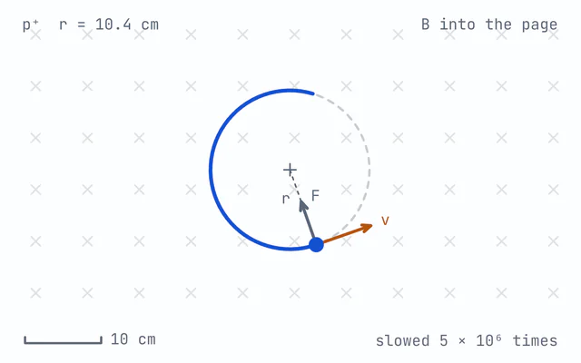
charged particle in a magnetic field simulator.
Neutral points, the classic plotting experiment
Lay a bar magnet on paper, plot its field with a compass, and somewhere the compass stops pointing anywhere in particular. There the magnet’s field exactly cancels Earth’s horizontal field: a neutral point. With the north end facing north, the two neutral points lie on the line across the magnet’s middle; for the 5 cm ferrite bar in a field of 20 µT, about London’s, they are 20.5 cm from its centre. Turn it round, north end facing south, and they move onto its axis, 26.1 cm out.
A point dipole puts them at (μ₀m/4πB)^(1/3) and (2μ₀m/4πB)^(1/3), 20.6 cm
and 26.0 cm: within 1 percent, and further out along the axis because a dipole’s field there is
twice as strong as across its middle. In Delhi’s stronger field of about 34 µT the magnet’s field
falls to Earth’s sooner, and the points move in to 17.1 cm and 22.0 cm. The scene finds every
neutral point in the area the probe can reach, outside the magnets, to below 10⁻¹² T, and marks it
with a cross.
Plotting a field line with a compass
The classroom method: put a small compass by the magnet, mark a dot where its north end points, move the compass on until its south end sits on that dot, and repeat. Trace with compass does just that, one needle-length of 2 cm at a time. Where the line curves tightly the dots drift off it, because each step runs straight along the direction where it began, which is Euler’s method and is why a smaller compass plots a truer line. The field lines drawn beside the dots are traced in steps of at most 4 mm by a fourth-order method. Round a lone magnet, coil or wire they stay within a micrometre of the true line, and in every arrangement offered here within a few hundredths of a millimetre, far less than a pixel.
What the spacing of the lines does and does not tell you
In three dimensions the number of field lines through each square metre is proportional to the field, which is why textbooks read strength from line density. This picture is a flat slice. The lines from each magnet and coil start at radii that would share out the flux through its middle equally if the field there were even, as it nearly is across a long bar magnet, but a slice cannot show them spreading out in space, so their spacing on the page is only a rough guide to the field, and lines from different magnets are not counted in proportion to their strength. A wire is the exception: its field is the same in every slice along it, and its lines are drawn at equal steps of flux, so they do crowd as 1/r. For the field itself, use the probe. The colour of the lines, and Strength, which shades the whole scene, show where it is stronger and weaker, on a logarithmic scale across what is in view.
Lines near a magnet’s axis close a long way out, often beyond the edge of the scene, and they are drawn to the edge rather than tidied into the neat ovals of a textbook sketch. The electric field simulator traces its lines the same way, but there they start on positive charges and end on negative ones. Magnetic field lines have no ends at all.
What this simulator leaves out
- Soft iron and changing magnets. Each magnet is rigid and uniformly magnetised, which suits ferrite and NdFeB but not alnico or a keeper of soft iron, and magnets never change one another’s magnetisation however close they are put.
- Forces. The pictures show the field, not how hard the magnets pull or twist, so two magnets drawn attracting are not being weighed.
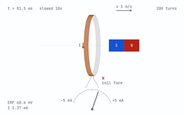
- Time. Every current is steady. Moving a magnet past a coil drives a current in it, which the electromagnetic induction simulator works out.
- The third dimension. Every magnet’s and coil’s axis lies in the page, wires are infinitely long and run straight through it, each coil’s turns share one plane, and Earth’s field is its horizontal part only.
Common mistakes
- Ending the lines at the south pole. They carry on through the magnet, from south to north, and close on themselves.
- Expecting a compass to point at a north pole. Unlike poles attract, so beside a magnet a compass’s north end points towards the magnet’s south pole.
- Reading strength from spacing in a flat picture. Use the probe: the spacing on the page is only a rough guide.
- Using the dipole formula close to a magnet. Three lengths from the centre of the 5 cm bar it is still 5.2 percent low along the axis and 4.0 percent high across the middle.
- Using
μ₀NI/(2R)anywhere but the centre of a coil. It is the field at the centre only. A Helmholtz pair is how a coil’s field is made even over a region.
Model and assumptions
- Method
- Exact expression, no time stepping
- Repeatability
- Deterministic. The same link gives the same numbers on any machine.
What it assumes
- Every current is steady, and the only magnetic material is the magnets themselves, so nothing else in the scene is magnetised by their field.
- Each magnet is rigid and uniformly magnetised along its axis, with a relative permeability of 1, which suits ferrite and NdFeB but not soft iron or alnico, and its field inside and out is that of a solenoid carrying Br/μ₀ amperes per metre, in Derby and Olbert’s closed form.
- Each coil is one circular loop carrying N times the current, its turns sharing one plane and one radius, with its exact field from complete elliptic integrals by the arithmetic-geometric mean.
- Wires are infinitely long and straight and run at right angles through the page, and every magnet’s and coil’s axis lies in it, so the field there has no part out of the page and the picture is an exact slice through the three-dimensional field.
- Earth’s field is its horizontal part only, uniform and pointing up the page to magnetic north, at the value set between 0 and 60 µT.
Where it stops holding. Magnets close enough to change each other’s magnetisation, soft iron such as a keeper or a core, alternating currents and the currents they induce, and the field away from the page itself, where a coil’s field has to be followed in three dimensions. The Solenoid Magnetic Field Simulator is the right tool there.
Numerical accuracy
No time stepping, so nothing accumulates. The readings at the probe and in the table are closed forms, exact to rounding: a wire’s μ₀I/2πr, a coil’s complete elliptic integrals by the arithmetic-geometric mean, and a bar magnet’s generalised elliptic integrals, after Bulirsch, in Derby and Olbert’s form. Two numbers are found by search: each neutral point, settled by Newton’s method on the exact field until the field there is below 10⁻¹² T, and a Helmholtz pair’s uniform length, found by halving an interval on the exact field until it is settled to the limit of double precision. Three pictures are approximate by construction. Each field line is traced in short steps along the field direction, a fourth-order Runge-Kutta step in distance rather than time, and stays within a micrometre of the true line round a lone magnet, coil or wire, and within a few hundredths of a millimetre in every preset, whose true lines are all known exactly. The iron filings are bent along the field by two midpoint steps either side of their middle, on the field sampled every 6 pixels, and the grid’s compass needles swing to the field with a damped rotation chosen for the eye, so no number is read from either. The plotting compass’s dots are the classroom method itself, one needle-length straight along the field at a time, and drift off the true line where it curves tightly, as a real compass’s do.
Constants used: Vacuum permeability (μ₀).
Common questions
How do you draw the magnetic field lines of a bar magnet?
Outside the magnet they leave the north pole and curve round to the south pole. Inside it they run from south to north, so every line is a closed loop. Here each line is traced through the exact field of a three-dimensional magnet, and the plotting compass draws one the classroom way: mark where its north end points, move it on so its south end sits on the mark, and repeat, a needle-length at a time.
Why do magnetic field lines never cross?
A field line points along the field, and the field has only one direction at each point. Two lines crossing would give that point two directions. Where lines seem to meet, at a neutral point, the field is zero and has no direction at all.
What is a neutral point?
A place where the fields cancel exactly, so the field there is zero and a compass points nowhere in particular. There is one between two like poles facing each other, and one between two wires carrying current the same way. In the classic plotting experiment they are where a magnet’s field exactly cancels Earth’s horizontal field: for a 5 cm by 1.2 cm ferrite bar in a 20 µT field with its north end facing north, there are two, 20.5 cm from its centre on the line across its middle. Turn the magnet round and they move onto its axis, 26.1 cm out. In Delhi’s stronger field of about 34 µT they move in to 17.1 cm and 22.0 cm.
What is the magnetic field around a current-carrying wire?
Circles round the wire, with B = μ₀I/2πr, pointing the way your fingers curl when your right thumb points along the current. A current of 10 A gives 40 µT at 5 cm, comparable to Earth’s field. Twice as far away, the field is half as strong.
How do you calculate the magnetic field of a Helmholtz coil?
Two identical coils of radius R placed R apart give B = (4/5)^(3/2) μ₀NI/R at the centre, which is 0.7155 times μ₀NI/R. With 100 turns of 10 cm radius carrying 1 A, that is 0.899 mT. Along the axis it stays within 1 percent of that value for 3.1 cm either side of the centre, which is why the pair is used to make a uniform field.
Does the spacing of the field lines show how strong the field is?
Only roughly, in a flat picture. The lines are exact paths through the three-dimensional field in the plane of the page, but in a slice they cannot thin out the way they do in space. To read the field itself, use the probe or turn on the strength shading.
Where is a bar magnet’s field strongest?
Inside the magnet, and round the edges of its ends, where the lines crowd round the corners and iron filings cluster. Along its axis the field of a 5 cm by 1.2 cm ferrite bar is 0.379 T at its centre, 0.194 T at the middle of its pole face and 27 mT a centimetre beyond it. That halving at the face is the same one the solenoid page explains.