Normal Distribution Calculator
Drag the bounds on a shaded bell curve for the probability, z-scores and full working, find any percentile, or fit a bell curve to pasted data.
Calculator
Drag along the axis to move the nearer bound. Or select the curve: the arrow keys move a bound 0.01σ, or 0.1σ with Shift, and Tab moves to the other one.
The chance that one value from N(100, 15²) lies between 85 and 115.
- P(85 < X < 115) The shaded area: the chance that one value drawn from this distribution lands there. The whole area under the curve is 1.
- 0.68269 68.269%
- z₁ at 85 How many standard deviations the bound lies from the mean, (x − μ) / σ. Negative below the mean.
- −1
- z₂ at 115 How many standard deviations the bound lies from the mean, (x − μ) / σ. Negative below the mean.
- 1
- Percentile of 85 The share of the distribution below the bound, 100Φ(z), as a percentile.
- 15.866th
- Percentile of 115 The share of the distribution below the bound, 100Φ(z), as a percentile.
- 84.134th
- Unshaded area The rest of the curve, worked out in its own tail rather than as 1 minus the shaded area, so it keeps its figures even when it is tiny.
- 0.31731
Working
- X ~ N(100, 15²). Standardise each bound with z = (x - μ) / σ, then read Φ(z), the area to the left of z.
- z₁ = (85 - 100) / 15 = -1
- z₂ = (115 - 100) / 15 = 1
- Φ(1) = 0.841345
- Φ(-1) = 0.158655
- P(85 < X < 115) = P(-1 < Z < 1) = Φ(1) - Φ(-1) = 0.841345 - 0.158655 = 0.68269
Citing this tool
Last updated . Add the date you accessed it as well, which a citation of a page that can change asks for. If a specific result matters, cite the permalink from the tool’s share row instead of this page: it reproduces the exact parameters.
The equation
The standard normal distribution; quantiles by Wichura (1988), Algorithm AS 241
What is the standard normal distribution Z-score formula?
The Z-score formula standardises any value x from a normal distribution with mean μ and standard deviation σ: z = (x − μ) / σ. The resulting z is the number of standard deviations x lies above or below the mean, and the standard normal cumulative distribution Φ(z) gives the probability of a value below x.
Normal probabilities in three steps
A normal distribution is fixed by two numbers, its mean μ and its standard deviation σ, and every normal curve is the same bell, shifted and stretched. That is why one function, Φ, answers every question about all of them, in three steps:
- Standardise. Turn each bound x into a z-score,
z = (x − μ) / σ, the number of standard deviations it lies from the mean. - Look up Φ(z), the area under the standard bell curve to the left of z, from a table or a calculator.
- Combine. Subtract two areas for a range,
P(a < X < b) = Φ(z_b) − Φ(z_a), and take an area from 1 for the part above a bound.
The whole area under the curve is 1, so every area is a probability: the chance that one value drawn from the distribution lands there. Going the other way, from an area back to a value, is the inverse normal, and the calculator prints its working too.
Using the calculator
Pick a question: Below, Above, Between, Outside or Percentile. Type the mean and the standard deviation, then drag along the axis or type the bounds, and the shading, its probability, both z-scores and the working follow. With the curve selected, the arrow keys move a bound by 0.01σ, or by 0.1σ with Shift, and Tab moves to the other bound. The 68-95-99.7 button marks the rule beneath the axis, z-table shows the row of a printed table for each bound, and Grade bands splits the curve into five. Save image gives a credited PNG of the curve as it stands, and the link keeps every setting.
Worked example: IQ-style scores, N(100, 15²)
Modern IQ tests, the Wechsler scales among them, are normed so that their scores have a mean of 100 and a standard deviation of 15, which is the curve the calculator opens with. That is a property of how the tests are scaled, and these are the areas it gives.
- Between 85 and 115.
z = (85 − 100) / 15 = −1andz = (115 − 100) / 15 = 1, soP(85 < X < 115) = Φ(1) − Φ(−1) = 0.841345 − 0.158655 = 0.68269, about 68.27 percent of scores. - Above 130.
z = (130 − 100) / 15 = 2andP(X > 130) = 1 − Φ(2) = 1 − 0.97725 = 0.02275, about 1 score in 44. - The 90th percentile.
z = Φ⁻¹(0.9) = 1.2816, sox = 100 + 1.2816 × 15 = 119.2.
Reading a z-table
A printed z-table gives Φ(z) to four decimals for z to two. Find the row for z to one decimal, then the column for its second decimal: for z = 1.28, row 1.2 and column 0.08 give 0.8997. For a negative z, use the symmetry Φ(−z) = 1 − Φ(z), so Φ(−1.00) = 1 − 0.8413 = 0.1587, or a table with negative rows. The calculator’s z-table button shows the row for each bound with its cell ringed, and the working uses the exact z rather than z rounded to two decimals.
| z | 0.00 | 0.01 | 0.02 | 0.03 | 0.04 | 0.05 | 0.06 | 0.07 | 0.08 | 0.09 |
|---|---|---|---|---|---|---|---|---|---|---|
| 0.0 | 0.5000 | 0.5040 | 0.5080 | 0.5120 | 0.5160 | 0.5199 | 0.5239 | 0.5279 | 0.5319 | 0.5359 |
| 0.1 | 0.5398 | 0.5438 | 0.5478 | 0.5517 | 0.5557 | 0.5596 | 0.5636 | 0.5675 | 0.5714 | 0.5753 |
| 0.2 | 0.5793 | 0.5832 | 0.5871 | 0.5910 | 0.5948 | 0.5987 | 0.6026 | 0.6064 | 0.6103 | 0.6141 |
| 0.3 | 0.6179 | 0.6217 | 0.6255 | 0.6293 | 0.6331 | 0.6368 | 0.6406 | 0.6443 | 0.6480 | 0.6517 |
| 0.4 | 0.6554 | 0.6591 | 0.6628 | 0.6664 | 0.6700 | 0.6736 | 0.6772 | 0.6808 | 0.6844 | 0.6879 |
| 0.5 | 0.6915 | 0.6950 | 0.6985 | 0.7019 | 0.7054 | 0.7088 | 0.7123 | 0.7157 | 0.7190 | 0.7224 |
| 0.6 | 0.7257 | 0.7291 | 0.7324 | 0.7357 | 0.7389 | 0.7422 | 0.7454 | 0.7486 | 0.7517 | 0.7549 |
| 0.7 | 0.7580 | 0.7611 | 0.7642 | 0.7673 | 0.7704 | 0.7734 | 0.7764 | 0.7794 | 0.7823 | 0.7852 |
| 0.8 | 0.7881 | 0.7910 | 0.7939 | 0.7967 | 0.7995 | 0.8023 | 0.8051 | 0.8078 | 0.8106 | 0.8133 |
| 0.9 | 0.8159 | 0.8186 | 0.8212 | 0.8238 | 0.8264 | 0.8289 | 0.8315 | 0.8340 | 0.8365 | 0.8389 |
| 1.0 | 0.8413 | 0.8438 | 0.8461 | 0.8485 | 0.8508 | 0.8531 | 0.8554 | 0.8577 | 0.8599 | 0.8621 |
| 1.1 | 0.8643 | 0.8665 | 0.8686 | 0.8708 | 0.8729 | 0.8749 | 0.8770 | 0.8790 | 0.8810 | 0.8830 |
| 1.2 | 0.8849 | 0.8869 | 0.8888 | 0.8907 | 0.8925 | 0.8944 | 0.8962 | 0.8980 | 0.8997 | 0.9015 |
| 1.3 | 0.9032 | 0.9049 | 0.9066 | 0.9082 | 0.9099 | 0.9115 | 0.9131 | 0.9147 | 0.9162 | 0.9177 |
| 1.4 | 0.9192 | 0.9207 | 0.9222 | 0.9236 | 0.9251 | 0.9265 | 0.9279 | 0.9292 | 0.9306 | 0.9319 |
| 1.5 | 0.9332 | 0.9345 | 0.9357 | 0.9370 | 0.9382 | 0.9394 | 0.9406 | 0.9418 | 0.9429 | 0.9441 |
| 1.6 | 0.9452 | 0.9463 | 0.9474 | 0.9484 | 0.9495 | 0.9505 | 0.9515 | 0.9525 | 0.9535 | 0.9545 |
| 1.7 | 0.9554 | 0.9564 | 0.9573 | 0.9582 | 0.9591 | 0.9599 | 0.9608 | 0.9616 | 0.9625 | 0.9633 |
| 1.8 | 0.9641 | 0.9649 | 0.9656 | 0.9664 | 0.9671 | 0.9678 | 0.9686 | 0.9693 | 0.9699 | 0.9706 |
| 1.9 | 0.9713 | 0.9719 | 0.9726 | 0.9732 | 0.9738 | 0.9744 | 0.9750 | 0.9756 | 0.9761 | 0.9767 |
| 2.0 | 0.9772 | 0.9778 | 0.9783 | 0.9788 | 0.9793 | 0.9798 | 0.9803 | 0.9808 | 0.9812 | 0.9817 |
| 2.1 | 0.9821 | 0.9826 | 0.9830 | 0.9834 | 0.9838 | 0.9842 | 0.9846 | 0.9850 | 0.9854 | 0.9857 |
| 2.2 | 0.9861 | 0.9864 | 0.9868 | 0.9871 | 0.9875 | 0.9878 | 0.9881 | 0.9884 | 0.9887 | 0.9890 |
| 2.3 | 0.9893 | 0.9896 | 0.9898 | 0.9901 | 0.9904 | 0.9906 | 0.9909 | 0.9911 | 0.9913 | 0.9916 |
| 2.4 | 0.9918 | 0.9920 | 0.9922 | 0.9925 | 0.9927 | 0.9929 | 0.9931 | 0.9932 | 0.9934 | 0.9936 |
| 2.5 | 0.9938 | 0.9940 | 0.9941 | 0.9943 | 0.9945 | 0.9946 | 0.9948 | 0.9949 | 0.9951 | 0.9952 |
| 2.6 | 0.9953 | 0.9955 | 0.9956 | 0.9957 | 0.9959 | 0.9960 | 0.9961 | 0.9962 | 0.9963 | 0.9964 |
| 2.7 | 0.9965 | 0.9966 | 0.9967 | 0.9968 | 0.9969 | 0.9970 | 0.9971 | 0.9972 | 0.9973 | 0.9974 |
| 2.8 | 0.9974 | 0.9975 | 0.9976 | 0.9977 | 0.9977 | 0.9978 | 0.9979 | 0.9979 | 0.9980 | 0.9981 |
| 2.9 | 0.9981 | 0.9982 | 0.9982 | 0.9983 | 0.9984 | 0.9984 | 0.9985 | 0.9985 | 0.9986 | 0.9986 |
| 3.0 | 0.9987 | 0.9987 | 0.9987 | 0.9988 | 0.9988 | 0.9989 | 0.9989 | 0.9989 | 0.9990 | 0.9990 |
| 3.1 | 0.9990 | 0.9991 | 0.9991 | 0.9991 | 0.9992 | 0.9992 | 0.9992 | 0.9992 | 0.9993 | 0.9993 |
| 3.2 | 0.9993 | 0.9993 | 0.9994 | 0.9994 | 0.9994 | 0.9994 | 0.9994 | 0.9995 | 0.9995 | 0.9995 |
| 3.3 | 0.9995 | 0.9995 | 0.9995 | 0.9996 | 0.9996 | 0.9996 | 0.9996 | 0.9996 | 0.9996 | 0.9997 |
| 3.4 | 0.9997 | 0.9997 | 0.9997 | 0.9997 | 0.9997 | 0.9997 | 0.9997 | 0.9997 | 0.9997 | 0.9998 |
Percentiles and the inverse normal
The inverse runs the steps backwards: from an area to a z with z = Φ⁻¹(p), then back to the scale with x = μ + zσ. Percentile mode takes the area to the left, to the right, in the middle or in both tails, typed as a decimal or a percent, or set by dragging the edge of the area. The central 95 percent of any normal curve lies within 1.95996 standard deviations of the mean, so for N(100, 15²) it runs from 70.6 to 129.4, and the same z leaves 2.5 percent in each tail. Φ⁻¹ is Wichura’s Algorithm AS 241 (1988), good to about one part in 10¹⁶.
Fitting a bell curve to your data
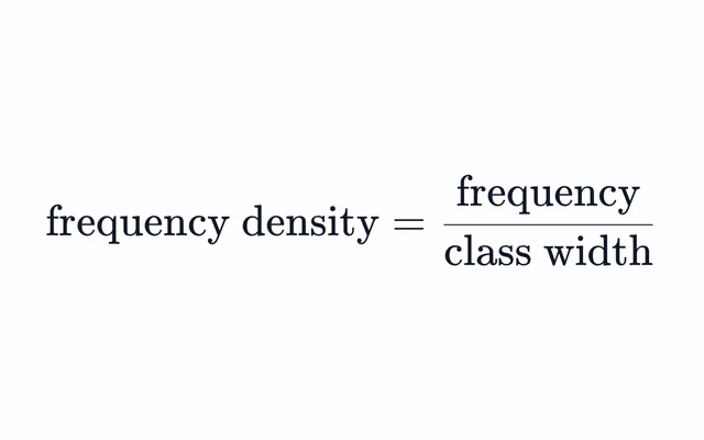
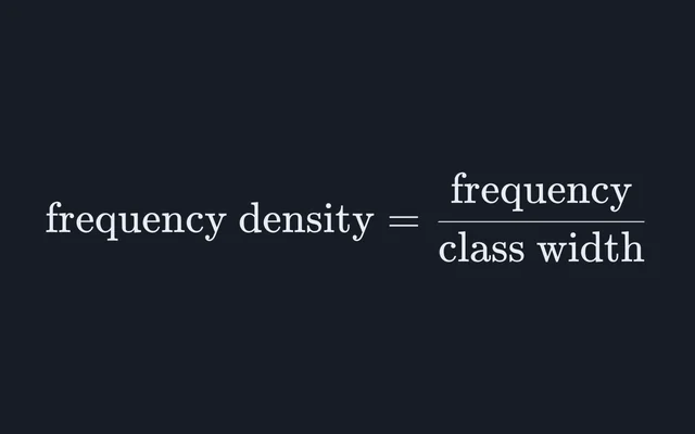
To make a bell curve from your own data, paste a column of numbers into the second tab, straight from a spreadsheet or typed with spaces or commas. The calculator finds their mean and standard deviation, the sample one by default, as the standard deviation calculator does, and draws a histogram on the density scale, where each bar’s area is its share of the data. The bars then add up to an area of 1, the same as the fitted curve, so the curve is drawn to the same scale as the bars and the two can be compared directly; the frequency density and histogram calculator explains the density scale. The number of bars follows the Freedman-Diaconis rule, bars about 2 × IQR × n^(−1/3) wide, and a slider changes it.
A histogram can look bell-shaped without being normal, so the tab adds a Q-Q plot, which puts each sorted value against the z a normal distribution would give it. Normal data lie along the straight line through the quartiles. The example’s 100 made-up test scores have a mean of 65.93 and a sample standard deviation of 13.75, and their lowest score, 27, sits about 6 below the line while their highest, 94, sits about 4 below it: a longer lower tail and a shorter upper one than a bell curve has, a slight left skew. Use this fit carries the mean and standard deviation to the probability tab.
Grading on a curve
Grading on a curve sets grade boundaries by position in the distribution rather than at fixed marks. With cut-offs at μ ± 0.5σ and μ ± 1.5σ, a normal curve splits into shares of 6.68, 24.17, 38.29, 24.17 and 6.68 percent, from E up to A. The Grade bands button draws those bands under the curve, lets you move each cut-off as a z or as a percentile, and in the data tab counts your own scores in each band beside what the fitted curve expects: for the example, 6, 23, 39, 24 and 8 against 6.68, 24.17, 38.29, 24.17 and 6.68.
Whether to grade on a curve at all is a policy decision for whoever sets the marks, and the calculator makes no recommendation. Real marks are often skewed, so a fixed share for each grade can mean very different marks from one test to the next, which a Q-Q plot of the marks themselves will show.
Common mistakes
- Using the variance for σ. A variance of 225 means σ = 15. Dividing by 225 instead gives z-scores fifteen times too small.
- Asking for P(X = a). One value has no width, so it has no area: P(X = 115) is 0, and P(X < 115) and P(X ≤ 115) are the same number, 0.84134.
- Forgetting to standardise. Φ(130) is not P(X < 130). A table is read at
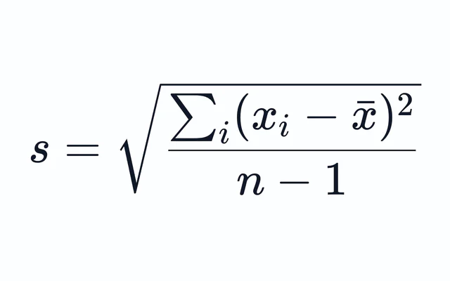
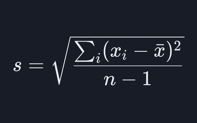
z = (130 − 100) / 15 = 2. - Mixing up the sample and population standard deviations. For data that are a sample of something larger, divide by n − 1. For the example scores that gives 13.75, against 13.68 dividing by n.
- Taking a far tail by subtraction.
1 − Φ(4)needs Φ(4) to nine figures to keep five in the answer, 3.1671 × 10⁻⁵. The calculator works out each tail in its own tail, which is how it givesP(5 < Z < 6) = 2.8566 × 10⁻⁷to every figure shown, where Φ(6) and Φ(5) agree to six decimal places.
Further tools
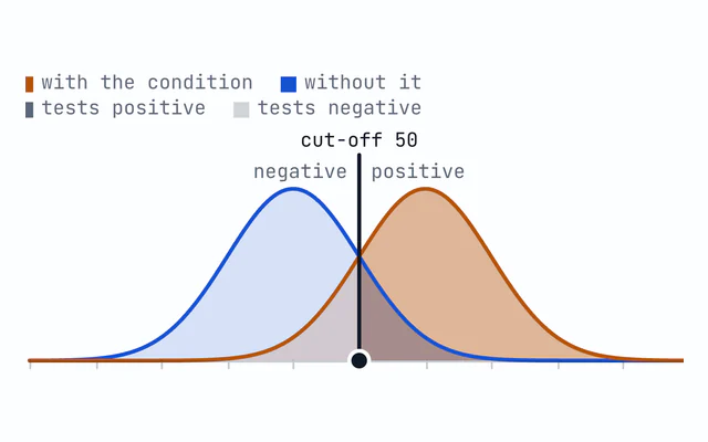
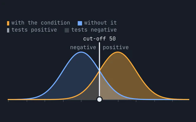
Two normal curves and a cut-off between them make the sensitivity and specificity visualiser, where the tails beyond the cut-off are the false positives and the false negatives. The chi-square calculator compares counts with the counts a ratio predicts, and the error propagation calculator combines standard deviations through a formula.
Common questions
How do you calculate a normal distribution probability step by step?
Standardise each bound with z = (x − μ)/σ, read Φ(z), the area to the left of z, from a table or a calculator, and combine the areas: subtract two of them for a range, or take one from 1 for the part above a bound. For IQ-style scores, N(100, 15²), P(X < 130) has z = (130 − 100)/15 = 2 and Φ(2) = 0.97725, so P(X > 130) = 1 − 0.97725 = 0.02275. Between 85 and 115 the z-scores are −1 and 1, and the area is 0.68269.
What is a z-score?
It is how many standard deviations a value lies from the mean, z = (x − μ)/σ, negative below the mean. On N(100, 15²) a score of 85 has z = (85 − 100)/15 = −1, and Φ(−1) = 0.15866, so 85 is at the 15.9th percentile: 15.9 percent of the distribution lies below it. A z-score puts values from different normal distributions on one scale, which is what lets one table serve them all.
What is the 68-95-99.7 rule?
In every normal distribution, 68.27 percent of values lie within 1 standard deviation of the mean, 95.45 percent within 2 and 99.73 percent within 3; to five decimal places they are 0.68269, 0.95450 and 0.99730. For N(100, 15²) that puts 68.27 percent of scores between 85 and 115 and 95.45 percent between 70 and 130. The middle 95 percent exactly lies within 1.95996 standard deviations, a little under 2.
How do I find the value at a given percentile?
Invert the distribution: find z = Φ⁻¹(p), the z with an area p to its left, then convert back with x = μ + zσ. For the 90th percentile of N(100, 15²), z = Φ⁻¹(0.9) = 1.2816 and x = 100 + 1.2816 × 15 = 119.2. The calculator’s Percentile mode does the same for an area to the right, in the middle or in both tails, with Φ⁻¹ from Wichura’s Algorithm AS 241.
How do I make a bell curve from my own data?
Paste the values into the calculator’s second tab. It draws a histogram on the density scale, so the bars’ total area is 1, overlays the normal curve with your data’s mean and standard deviation, and adds a Q-Q plot that shows how normal the data really are, since normal data lie along its straight line. The 100 example scores give a mean of 65.93, a sample standard deviation of 13.75 and 10 bars by the Freedman-Diaconis rule. Use this fit then carries the mean and standard deviation to the probability tab.
How does grading on a curve work?
Grade boundaries are set by position in the distribution, in standard deviations from the mean or as percentiles, rather than at fixed marks. With cut-offs at ±0.5σ and ±1.5σ, a normal curve gives shares of 6.7, 24.2, 38.3, 24.2 and 6.7 percent from the lowest band to the highest. Whether to curve at all is a policy decision rather than something the maths settles, and real scores are often skewed, which the calculator’s Q-Q plot of your own marks will show.
Why is the probability of one exact value zero?
A single value has no width, so it has no area under the curve, and for a continuous distribution probability is area. That is why P(X ≤ a) and P(X < a) are the same number: for N(100, 15²) both P(X ≤ 115) and P(X < 115) are 0.84134. To ask about a whole-number score of exactly 115, ask about the interval it stands for, P(114.5 < X < 115.5), which is 0.016131.