Spearman’s Rank Correlation Calculator
Paste paired data for Spearman’s rank correlation coefficient, with tied values given average ranks, the ranks table and an exact or t-based p-value.
Calculator
Two columns, x first and then y, one pair per line. Paste them from a spreadsheet or type them separated by tabs, commas or spaces. A first line of column names labels the table.
11 pairs read.
- Each pair’s ranks
- rs From −1, the ranks in exactly opposite order, through 0, no tendency, to 1, the same order.
- 0.818
- Pairs, n
- 11
- Σd² The sum of the squared differences between each pair’s two ranks.
- 40
- p, two-tailed The probability of an rs at least this far from zero if there were no association between the ranks. It is not the probability that there is none.
- 0.00208
- Method Above 10 pairs, t = rs √((n − 2)/(1 − rs²)) on n − 2 degrees of freedom. It runs slightly low with few pairs, so check a result close to α against a table of critical values.
- t approximation, 9 degrees of freedom
- t
- 4.269
- Degrees of freedom
- 9
Significant at α = 0.05. With rs = 0.818, the p-value, 0.00208 (from the t approximation), is at or below α, so reject the null hypothesis of no correlation between the ranks: the ranks tend to rise together.
Ranks for each pair
| x | Rank | y | Rank | d | d² |
|---|---|---|---|---|---|
| 10 | 7 | 8.04 | 7 | 0 | 0 |
| 8 | 5 | 6.95 | 4 | 1 | 1 |
| 13 | 10 | 7.58 | 6 | 4 | 16 |
| 9 | 6 | 8.81 | 9 | −3 | 9 |
| 11 | 8 | 8.33 | 8 | 0 | 0 |
| 14 | 11 | 9.96 | 10 | 1 | 1 |
| 6 | 3 | 7.24 | 5 | −2 | 4 |
| 4 | 1 | 4.26 | 1 | 0 | 0 |
| 12 | 9 | 10.84 | 11 | −2 | 4 |
| 7 | 4 | 4.82 | 2 | 2 | 4 |
| 5 | 2 | 5.68 | 3 | −1 | 1 |
| Σd² | 40 | ||||
Working
- n = 11
- Σd² = 40, where d = rank of x − rank of y
- rs = 1 − 6Σd² / (n(n² − 1)) = 1 − 6 × 40 / (11 × 120) = 0.81818
- t = rs √((n − 2) / (1 − rs²)) = 0.81818 × √(9 / (1 − 0.81818²)) = 4.2691
- p, two-tailed = P(|rs| ≥ 0.81818), by the t approximation on 9 degrees of freedom = 0.00208
- p = 0.00208 ≤ 0.05: significant at α = 0.05
Citing this tool
Last updated . Add the date you accessed it as well, which a citation of a page that can change asks for. If a specific result matters, cite the permalink from the tool’s share row instead of this page: it reproduces the exact parameters.
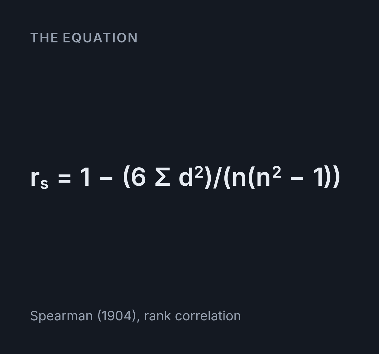
The equation
Spearman (1904), rank correlation
How do you calculate Spearman’s rank correlation coefficient?
Rank each variable separately, 1 for the smallest, giving tied values the average of the ranks they span. For each pair, subtract one rank from the other to get d, then square and add: rs = 1 − 6Σd²/(n(n² − 1)), where n is the number of pairs. rs runs from −1, opposite orders, to 1, the same order.
Worked example: Anscombe’s first data set
The calculator opens on the first of Anscombe’s four sets of eleven points (Anscombe 1973, The American Statistician 27: 17 to 21). Ranked separately and paired up again, its ranks give:
n = 11Σd² = 40, where d = rank of x − rank of yrs = 1 − 6Σd² / (n(n² − 1)) = 1 − 6 × 40 / (11 × 120) = 0.81818t = rs √((n − 2) / (1 − rs²)) = 0.81818 × √(9 / (1 − 0.81818²)) = 4.2691p, two-tailed = P(|rs| ≥ 0.81818), by the t approximation on 9 degrees of freedom = 0.00208p = 0.00208 ≤ 0.05: significant at α = 0.05
An APA-style report would read rs(9) = .82, p = .002, with n − 2 = 9 in the brackets. With eleven pairs the p-value comes from the t approximation. At 10 pairs or fewer the calculator counts every ordering of the ranks instead, as the section on exact p-values explains.
Tied values
Equal values share a rank: each takes the average of the positions they occupy, so 10, 20, 20, 30 rank 1, 2.5, 2.5, 4. Anscombe’s fourth set is the extreme case. 10 of its eleven x values are 8, so each ranks 5.5, and the one value of 19 ranks 11.
The short formula assumes the ranks are 1 to n with no repeats, so with ties it is only an approximation. On the fourth set it gives 0.625, while Pearson’s r calculated on the averaged ranks, the definition the short formula comes from, gives 0.500. The calculator reports the second, which is what R and SciPy report, and shows the first in the working for comparison with a mark scheme.
Spearman’s rs and Pearson’s r
Pearson’s r measures how close the points lie to a straight line, and rs measures only whether the two orders agree. That makes rs the better choice for a relationship that rises steadily but not in a straight line, for data that are themselves ranks or ordered categories, and for data with an outlier. Anscombe’s third set is ten points almost exactly on a straight line and one far above it. The outlier holds Pearson’s r to 0.816, but it moves only one place in the ranking, so Σd² = 2 and rs = 0.991. The linear regression calculator gives Pearson’s r with the line itself.
Exact p-values and the t approximation
If the two variables are unrelated, every ordering of one set of ranks against the other is equally likely, so the exact p-value is a count: the share of all n! orderings that give an rs at least as extreme as the one observed. Up to 10 pairs the calculator makes that count, ties included, which is how printed tables of critical values for small samples are worked out. Above 10 it uses t = rs √((n − 2)/(1 − rs²)) on n − 2 degrees of freedom, and the result names the method it used.
The approximation runs slightly low with few pairs, so check a borderline result against the table your course uses. At 11 pairs, an rs of 0.618 has an exact two-tailed p-value of 0.0478 and the next attainable value below it, 0.609, has 0.0519, so 0.618 is the exact critical value at 0.05. The t approximation gives 0.609 a p-value of 0.0467 and calls anything from 0.602 upward significant. Ranks in perfect order are the one case above 10 pairs that stays exact, because the orderings that reach rs = 1 or −1 can be counted directly.
Critical values of Spearman’s rs
A result is significant when rs, or −rs for a predicted negative correlation, is at or above the value for its number of pairs. Each value is the smallest rs whose exact probability is at most α, from the same count the calculator makes, and the tests check them against Zar (1972, Journal of the American Statistical Association 67: 578 to 580). The table starts at 5 pairs. Where it says n/a, no rs is that rare, not even 1.
| Pairs, n | 0.05 (0.10) | 0.025 (0.05) | 0.01 (0.02) | 0.005 (0.01) |
|---|---|---|---|---|
| 5 | 0.900 | 1.000 | 1.000 | n/a |
| 6 | 0.829 | 0.886 | 0.943 | 1.000 |
| 7 | 0.714 | 0.786 | 0.893 | 0.929 |
| 8 | 0.643 | 0.738 | 0.833 | 0.881 |
| 9 | 0.600 | 0.700 | 0.783 | 0.833 |
| 10 | 0.564 | 0.648 | 0.745 | 0.794 |
Common mistakes
- Ranking the two variables in opposite directions. Rank both from smallest to largest, or both from largest to smallest. Mixing the two flips the sign of rs.
- Giving tied values different ranks. Equal values must share the average rank. Ranking them 2 and 3 in the order they happen to be written makes rs depend on the order of the rows.
- Taking n as the number of values. n is the number of pairs, so ten pairs are twenty values and n = 10.
- Reading rs as cause and effect. A strong rank correlation says the two orders agree, not that one variable drives the other. Both can follow a third.
- Choosing a one-tailed test after seeing the sign of rs. Predict the direction before collecting the data, or use the two-tailed test.
What this calculator leaves out
It gives Spearman’s rs and its test, and nothing else: not Kendall’s tau, a confidence interval for rs, or a partial correlation that holds a third variable fixed. To ask whether two groups’ means differ, rather than whether two variables move together, use the t-test calculator. Counts in categories need the chi-square calculator, and the spread of a single variable the standard deviation calculator.
Common questions
How do you rank tied values in Spearman’s rank?
Give each tied value the average of the ranks the tied values would have taken. In 10, 20, 20, 30 the two 20s would be ranks 2 and 3, so each gets 2.5, and 30 is still rank 4. With ties the short formula 1 − 6Σd²/(n(n² − 1)) is only approximate, so the calculator reports Pearson’s r between the ranks, as R and SciPy do, and shows the short formula beside it.
How do you know if Spearman’s rank is significant?
Compare rs with the critical value for your number of pairs, or read its p-value. Two-tailed at 0.05, rs must reach 0.738 with 8 pairs and 0.648 with 10. Up to 10 pairs this calculator counts every possible ordering of the ranks for an exact p-value. Above 10 it uses t = rs √((n − 2)/(1 − rs²)) on n − 2 degrees of freedom and says so.
What does a negative Spearman’s rank correlation mean?
That as one variable’s rank rises, the other’s tends to fall. rs runs from −1, where one order is the exact reverse of the other, through 0, no tendency either way, to 1, where the two orders agree completely. Its sign gives the direction and its size the strength, while whether it is significant depends on the number of pairs as well.
When should I use Spearman’s rank instead of Pearson’s r?
When the relationship rises or falls steadily but not in a straight line, when the data are ranks or ordered categories, or when an outlier would dominate Pearson’s r. Anscombe’s third data set is ten points almost exactly on a line and one far above it: the outlier holds Pearson’s r to 0.816, but it moves only one place in the ranking, so rs is 0.991.