T-Test Calculator
Run a one-sample, two-sample (Welch or pooled) or paired t-test from raw data or summary statistics, with t, degrees of freedom, p-values and working.
Calculator
10 values read.
10 values read.
Paste a column from a spreadsheet, or type values separated by spaces, commas or new lines.
- t The difference between the two means divided by its standard error.
- −2.134
- Degrees of freedom From the Welch-Satterthwaite equation, so usually not a whole number.
- 16.786
- p, two-tailed P(|T| ≥ |t|). The probability of a t at least this far out if the null hypothesis were true. It is not the probability that the null hypothesis is true.
- 0.0479
- p, one-tailed (μ₁ < μ₂) Half the two-tailed p-value when t points the way predicted. Use it only when the direction was fixed before the data were seen.
- 0.0239
- Critical t, α = 0.05 The t that leaves α/2 in each tail. A |t| at or beyond it is significant.
- ±2.112
- 95% confidence interval for μ₁ − μ₂ Always two-sided. It excludes the null value exactly when the two-tailed test at the same α is significant.
- −0.9829 to −0.005128
Significant at α = 0.05. |t| = 2.134 is at or above the two-tailed critical value of 2.112, so reject the null hypothesis that the two population means are equal. If it were true, a t at least this far from zero would turn up with probability 0.0479.
| n | Mean | SD | SE of the mean | |
|---|---|---|---|---|
| Group 1 | 10 | 5.032 | 0.5831 | 0.1844 |
| Group 2 | 10 | 5.526 | 0.4426 | 0.14 |
- t distribution, 16.786 degrees of freedom
- Critical values at α = 0.05
- t = −2.134
Working
- group 1: n₁ = 10, x̄₁ = 5.032, s₁ = 0.58309
- group 2: n₂ = 10, x̄₂ = 5.526, s₂ = 0.44257
- SE = √(s₁²/n₁ + s₂²/n₂) = √(0.58309²/10 + 0.44257²/10) = 0.23149
- t = (x̄₁ − x̄₂) / SE = (5.032 − 5.526) / 0.23149 = −2.134
- df = (s₁²/n₁ + s₂²/n₂)² / [(s₁²/n₁)²/(n₁ − 1) + (s₂²/n₂)²/(n₂ − 1)] = 0.053587² / (0.034²/9 + 0.019587²/9) = 16.786
- p, two-tailed = P(|T| ≥ 2.134) on 16.786 degrees of freedom = 0.0479
- critical t at α = 0.05, two-tailed = 2.112
- 95% confidence interval = −0.494 ± 2.1119 × 0.23149 = −0.98287 to −0.0051279
- |t| = 2.134 ≥ 2.112, so p ≤ 0.05: significant at α = 0.05
Citing this tool
Last updated . Add the date you accessed it as well, which a citation of a page that can change asks for. If a specific result matters, cite the permalink from the tool’s share row instead of this page: it reproduces the exact parameters.
The equation
Student (1908), with Welch (1947) for unequal variances
What is the t-test formula?
A t-test divides a difference between means by its standard error. For one sample, t = (x̄ − μ₀)/(s/√n), with n − 1 degrees of freedom. For two independent samples, Welch’s test uses t = (x̄₁ − x̄₂)/√(s₁²/n₁ + s₂²/n₂). The p-value is the probability of a t this far from zero if the null hypothesis is true.
Which t-test to use
- One sample compares a sample’s mean with a value fixed before the data were collected, such as a stated fill volume or a theoretical value. It has n − 1 degrees of freedom.
- Paired is for two measurements on each subject: before and after a treatment, two drugs given to the same patients, or the left and right sides of the same body. It subtracts each pair and runs a one-sample test on the differences against zero, with one fewer degree of freedom than there are pairs.
- Two samples is for two separate groups of individuals. Welch’s test, the default here, lets each group keep its own variance and takes its degrees of freedom from the Welch-Satterthwaite equation, so they are usually not a whole number. The pooled test, Student’s original, assumes the two populations share one variance and has n₁ + n₂ − 2 degrees of freedom.
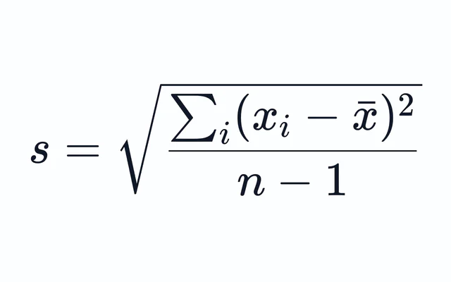
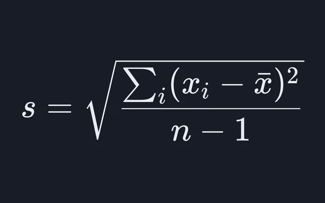
Every version needs the same three figures from each sample, its mean, its standard deviation and its size, which is why the calculator works from summary statistics as well as from raw data. For the spread of a single column, with the standard error and a confidence interval for its mean, use the standard deviation calculator.
Worked example: two groups of plants
The calculator opens on the dried weights of ten plants grown as a control and ten grown under a treatment (Dobson 1983, An Introduction to Statistical Modelling, distributed with R as PlantGrowth): 4.17, 5.58, 5.18, 6.11, 4.50, 4.61, 5.17, 4.53, 5.33, 5.14 for the control, and 6.31, 5.12, 5.54, 5.50, 5.37, 5.29, 4.92, 6.15, 5.80, 5.26 under the treatment.
- Control:
x̄₁ = 5.032,s₁ = 0.5831. Treatment:x̄₂ = 5.526,s₂ = 0.4426. - Standard error of the difference:
√(s₁²/10 + s₂²/10) = 0.2315. t = (5.032 − 5.526) / 0.2315 = −2.134, on 16.786 degrees of freedom from the Welch-Satterthwaite equation.- The two-tailed critical value at α = 0.05 is 2.112, and the p-value is 0.0479.
So the difference is significant at 0.05, though only just, and a report would read t(16.79) = −2.13, p = .048. The 95% confidence interval for μ₁ − μ₂ runs from −0.9829 to −0.005128. It excludes zero, as it must when the two-tailed test is significant, but only barely, so the data are also consistent with a very small difference.
The pooled test gives the same t here, because the groups are the same size, but its 18 degrees of freedom give a p-value of 0.0469. With equal group sizes the two tests rarely disagree by much. With unequal sizes and unequal spreads they can, and it is the pooled test whose false-positive rate then drifts away from α, which is why Welch’s test is the default (Ruxton 2006, Behavioral Ecology 17: 688 to 690).
Worked example: why pairing matters
Student’s 1908 paper analyzed the extra hours of sleep that ten patients gained, against a control night, on each of two drugs (Cushny and Peebles 1905). Every patient took both drugs, so the data are paired by patient. Choose Paired in the calculator and it opens on them:
differences, d = measurement 1 − measurement 2: −1.2, −2.4, −1.3, −1.3, 0, −1, −1.8, −0.8, −4.6, −1.4n = 10, d̄ = −1.58, s_d = 1.23SE = s_d / √n = 1.23 / √10 = 0.38896t = (d̄ − μ₀) / SE = (−1.58 − 0) / 0.38896 = −4.0621df = n − 1 = 9p, two-tailed = P(|T| ≥ 4.0621) on 9 degrees of freedom = 0.00283critical t at α = 0.05, two-tailed = 2.26295% confidence interval = −1.58 ± 2.2622 × 0.38896 = −2.4599 to −0.70011|t| = 4.062 ≥ 2.262, so p ≤ 0.05: significant at α = 0.05
Enter the same twenty numbers as two independent groups and Welch’s test gives t = −1.861 and p = 0.0794, not significant. Patients who slept well on one drug tended to sleep well on the other, so much of the spread within each column belongs to the patients rather than to the drugs. The paired test works on the differences, which removes it: the standard error falls from 0.8491 hours to 0.389. The pairing has to come from how the data were collected, though. Matching values that were never measured on the same subject is as wrong as ignoring a real pairing.
One-tailed or two-tailed?
A two-tailed test asks whether the means differ in either direction. A one-tailed test asks about one direction only, and it is valid only when that direction was stated before the data were seen and a difference the other way would count the same as none. On the plant weights, a prediction that the treated plants are heavier, μ₁ < μ₂, gives a one-tailed p-value of 0.0239, half the two-tailed 0.0479, against a one-tailed critical value of −1.741. Choosing the tail after seeing which way the data went doubles the false-positive rate, because either tail could have been the one chosen.
What the test assumes
- Independent observations. Each value, or each pair, comes from a different subject, and none influences another. Repeated measurements on one subject entered as separate values break this, and no choice of t-test repairs it.
- Normal populations, or samples large enough not to need them. The t distribution is exact for normally distributed data, and by the central limit theorem it becomes a good approximation for other shapes as the samples grow. With small samples, strong skew or outliers it can mislead, and a rank-based test such as the Mann-Whitney U test or the Wilcoxon signed-rank test is the usual alternative.
- Equal variances, for the pooled test only. Welch’s test drops this assumption, and loses very little when the variances do turn out to be equal.
Critical values of the t distribution
A two-tailed test at level α is significant when |t| is at or above the value in the column for that two-tailed α. A one-tailed test is significant when t is at or beyond the value in the column for its one-tailed α, in the predicted direction. The table runs to 120 degrees of freedom; the calculator gives the value for any number, including Welch’s fractional ones.
| Degrees of freedom | 0.10 (0.20) | 0.05 (0.10) | 0.025 (0.05) | 0.01 (0.02) | 0.005 (0.01) | 0.0005 (0.001) |
|---|---|---|---|---|---|---|
| 1 | 3.078 | 6.314 | 12.706 | 31.821 | 63.657 | 636.619 |
| 2 | 1.886 | 2.920 | 4.303 | 6.965 | 9.925 | 31.599 |
| 3 | 1.638 | 2.353 | 3.182 | 4.541 | 5.841 | 12.924 |
| 4 | 1.533 | 2.132 | 2.776 | 3.747 | 4.604 | 8.610 |
| 5 | 1.476 | 2.015 | 2.571 | 3.365 | 4.032 | 6.869 |
| 6 | 1.440 | 1.943 | 2.447 | 3.143 | 3.707 | 5.959 |
| 7 | 1.415 | 1.895 | 2.365 | 2.998 | 3.499 | 5.408 |
| 8 | 1.397 | 1.860 | 2.306 | 2.896 | 3.355 | 5.041 |
| 9 | 1.383 | 1.833 | 2.262 | 2.821 | 3.250 | 4.781 |
| 10 | 1.372 | 1.812 | 2.228 | 2.764 | 3.169 | 4.587 |
| 11 | 1.363 | 1.796 | 2.201 | 2.718 | 3.106 | 4.437 |
| 12 | 1.356 | 1.782 | 2.179 | 2.681 | 3.055 | 4.318 |
| 13 | 1.350 | 1.771 | 2.160 | 2.650 | 3.012 | 4.221 |
| 14 | 1.345 | 1.761 | 2.145 | 2.624 | 2.977 | 4.140 |
| 15 | 1.341 | 1.753 | 2.131 | 2.602 | 2.947 | 4.073 |
| 16 | 1.337 | 1.746 | 2.120 | 2.583 | 2.921 | 4.015 |
| 17 | 1.333 | 1.740 | 2.110 | 2.567 | 2.898 | 3.965 |
| 18 | 1.330 | 1.734 | 2.101 | 2.552 | 2.878 | 3.922 |
| 19 | 1.328 | 1.729 | 2.093 | 2.539 | 2.861 | 3.883 |
| 20 | 1.325 | 1.725 | 2.086 | 2.528 | 2.845 | 3.850 |
| 21 | 1.323 | 1.721 | 2.080 | 2.518 | 2.831 | 3.819 |
| 22 | 1.321 | 1.717 | 2.074 | 2.508 | 2.819 | 3.792 |
| 23 | 1.319 | 1.714 | 2.069 | 2.500 | 2.807 | 3.768 |
| 24 | 1.318 | 1.711 | 2.064 | 2.492 | 2.797 | 3.745 |
| 25 | 1.316 | 1.708 | 2.060 | 2.485 | 2.787 | 3.725 |
| 26 | 1.315 | 1.706 | 2.056 | 2.479 | 2.779 | 3.707 |
| 27 | 1.314 | 1.703 | 2.052 | 2.473 | 2.771 | 3.690 |
| 28 | 1.313 | 1.701 | 2.048 | 2.467 | 2.763 | 3.674 |
| 29 | 1.311 | 1.699 | 2.045 | 2.462 | 2.756 | 3.659 |
| 30 | 1.310 | 1.697 | 2.042 | 2.457 | 2.750 | 3.646 |
| 40 | 1.303 | 1.684 | 2.021 | 2.423 | 2.704 | 3.551 |
| 60 | 1.296 | 1.671 | 2.000 | 2.390 | 2.660 | 3.460 |
| 100 | 1.290 | 1.660 | 1.984 | 2.364 | 2.626 | 3.390 |
| 120 | 1.289 | 1.658 | 1.980 | 2.358 | 2.617 | 3.373 |
Every figure is computed by the function the calculator uses, which the tests check against the NIST/SEMATECH e-Handbook of Statistical Methods and against Fisher and Yates’ tables.
Common mistakes
- Entering the standard error as the standard deviation. A paper that reports mean ± SEM has already divided the standard deviation by √n, so multiply back: SD = SEM × √n. Entered as it stands, the SEM makes t √n times too large.
- A two-sample test on paired data. On the sleep data it turns a p-value of 0.00283 into 0.0794.
- Reading “not significant” as “no difference”. A p-value above α says the data are consistent with no difference, not that the means are equal. A small sample can miss a real difference, and the confidence interval shows how large a difference the data still allow.
- Running a t-test on every pair of three or more groups. Each comparison carries its own chance of a false positive, and the chances add up across the comparisons. A one-way analysis of variance tests all the groups at once.
- Testing counts in categories. A t-test compares the means of measurements. Counts, such as offspring of each phenotype, need the chi-square calculator.
What this calculator leaves out
It runs the one-sample, paired and two-sample t-tests and nothing else: not the analysis of variance for three or more groups, the rank-based tests for data far from normal, equivalence tests, or power and sample-size calculations. To ask whether two measured variables rise and fall together, rather than whether two means differ, the Spearman’s rank correlation calculator tests an association between ranks, and the linear regression calculator fits a line.
Common questions
Which t-test should I use?
Use a paired t-test when each value in one set is matched to one in the other, such as the same patients measured before and after a treatment, and a two-sample test when the two groups are different individuals. A one-sample test compares one mean with a fixed value stated in advance. A two-sample test run on paired data throws the pairing away: on Student’s sleep data it gives p = 0.079 where the paired test gives p = 0.0028.
What is the difference between Welch’s t-test and Student’s t-test?
Student’s two-sample test pools the two sample variances into one estimate, which assumes the populations share a variance, and has n₁ + n₂ − 2 degrees of freedom. Welch’s test keeps each sample’s own variance and takes its degrees of freedom from the Welch-Satterthwaite equation, usually a fraction. When the variances and the group sizes both differ, the pooled test’s false-positive rate can sit well away from α while Welch’s stays close to it, so Welch’s is the default here, as it is in R.
Should I use a one-tailed or a two-tailed t-test?
Use a two-tailed test unless the direction of the difference was predicted before the data were collected, and a difference the other way would be treated the same as no difference at all. When the result goes the predicted way the one-tailed p-value is half the two-tailed one, so choosing the tail after seeing the data doubles the false-positive rate.
What is the critical value of t at the 0.05 level?
It depends on the degrees of freedom and on the tails. Two-tailed at 0.05 it is 12.706 at 1 degree of freedom, 2.262 at 9, 2.086 at 20 and 2.042 at 30, falling toward the normal distribution’s 1.960 as the degrees of freedom grow. One-tailed at 0.05 the same rows give 6.314, 1.833, 1.725 and 1.697. The table on this page runs to 120 degrees of freedom, and the calculator gives the value for any number.
Can I run a t-test from the mean and standard deviation alone?
Yes. A t-test needs only each sample’s mean, standard deviation and size, so choose Summary statistics and type them in. Use the sample standard deviation, with n − 1 in its denominator, not the standard error of the mean: a paper that reports mean ± SEM gives the standard deviation as SEM × √n.