Color Blindness Simulator
Upload an image or screenshot and see it as red-green or blue-yellow colour blind eyes do, from mild to complete. Your image never leaves your device.
Simulator
Drop, paste or choose an image
Opened on this device and sent nowhere.
Drag the divider or use the arrow keys, Home and End. Hold the picture, or O, to see the original; hover or tap for the loupe. Space plays and pauses.
Berries in leaves: clusters of red berries on a sprig of green leaves, simulated for deuteranopia. The hardest pair to tell apart is #5a7a37 and #a32e2d: a colour difference of 72 in typical vision falls to 6. The picture keeps 68 percent of its colour difference. The spectrum turns grey at 500 nm, the neutral point.
The hardest pair in this picture
#5a7a37 and #a32e2d
- Hardest pair Of the picture’s six main colours, the two that lose most of their difference: #5a7a37 and #a32e2d, 72.1 apart in typical vision and 6.2 apart with deuteranopia, in CIELAB delta E. Under 10 is hard to tell apart at a glance.
- 72 → 6 ΔE
- Colour difference kept The colour difference between two points of the picture picked at random, on average, as a share of what it is in typical vision. Worked out on the picture’s six main colours, each weighted by how much of the picture it covers.
- 68 %
- Cone shift How far the anomalous cone’s curve has slid towards the other: Machado and colleagues take 20 nm as the shift at which the two almost coincide, which is 100 percent.
- +20 nm
- How common Deuteranopia: 1.27 percent of men and 0.01 percent of women of European ancestry, about 1 in 10,000 women, from the figures Sharpe and colleagues (1999) gathered. Red-green rates are lower in many other populations.
- 1 in 79 men
Drag along the chart, or use the arrow keys, to slide the M curve and set the severity. Each curve is drawn in the colour of the light at its peak: L solid, M dashed, S dotted.
On this picture the two differ by ΔE 1.4 on average, about the smallest difference people notice.
Citing this tool
Last updated . Add the date you accessed it as well, which a citation of a page that can change asks for. If a specific result matters, cite the permalink from the tool’s share row instead of this page: it reproduces the exact parameters.
On the syllabus: MCAT, 6A: Sensing the environment.
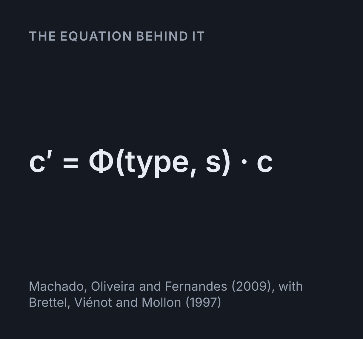
The equation
Machado, Oliveira and Fernandes (2009), with Brettel, Viénot and Mollon (1997)
What are the common types of colour vision deficiency?
Colour vision deficiency (colour blindness) usually comes from an inherited change in one cone photopigment, shifted in an anomaly or missing in an anopia: deuteranomaly/deuteranopia, the most common, affects green cones (M cones), protanomaly/protanopia affects red cones (L cones), and tritanomaly/tritanopia affects blue cones (S cones).
What a colour blindness simulator shows
A colour blindness simulator redraws a picture as it is likely to look to someone whose cones respond differently from most people’s. This one takes any image you drop, paste or choose, or one of six built-in pictures, and shows it with a protan (L cone), deutan (M cone) or tritan (S cone) deficiency at any severity from 0 to 100 percent. Your image is decoded and simulated by this page in your browser and sent nowhere.
Every pixel goes through the same three steps: its sRGB value is decoded to linear light, multiplied by a 3 by 3 matrix for the deficiency, and encoded back. Below 100 percent the matrices are the 33 that Machado, Oliveira and Fernandes published in 2009, blended between their tenths; at 100 percent tritan the simulator switches to the method of Brettel, Viénot and Mollon (1997), and for complete protan and deutan you can compare the two. It is a demonstration, not a diagnosis: a screen cannot tell you whether you are colour blind, and nothing here asks what you see. An optometrist can test colour vision properly.
How to read the wipe and the cone chart
Left of the divider is the picture as typical vision sees it, right of it the simulation. Drag the divider, or focus the picture and use the arrow keys, Home and End. Press and hold the picture, or hold O, to see the original everywhere; tap it, or hover over it with a mouse, and the loupe gives one pixel’s hex code before and after with the colour difference between them. Side by side puts the two in full, and Three-up shows protan, deutan and tritan at once beside typical vision, which is the quickest way to check a design.
The cone chart under the picture is why the picture changes. It plots the three cone sensitivities from 380 to 700 nm, computed from the CIE 1931 colour matching functions through Smith and Pokorny’s transform, and each curve is drawn in the colour of the light at its own peak: L, solid, at 567 nm, M, dashed, at 543 nm and S, dotted, at 448 nm. Measured in the eye, they peak nearer 565, 545 and 440 nm; the 1931 functions place the S peak a few nanometres long. The so-called red cone peaks in the yellow-green. Red looks red because it excites L far more than M, so it is the gap between those two curves that carries red against green. Move the severity and the affected curve slides towards its neighbour, leaving a faint ghost where it was, and the arrow above gives the shift in nanometres; drag the curve itself and the severity follows.
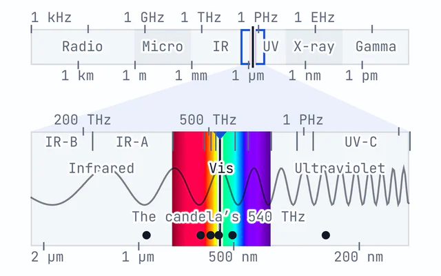
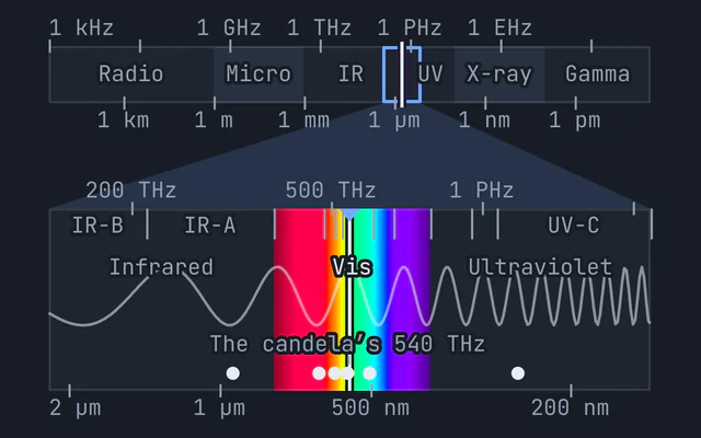
Under the curves are two strips: the spectrum as typical vision sees it, and as the chosen deficiency does. With the M cone gone the red-green axis collapses and the second strip runs from blue through grey to yellow, grey exactly where the caret marks the neutral point: 494 nm for protanopia, 500 nm for deuteranopia and 566 nm for tritanopia in this simulation. An anomalous trichromat has no neutral point, only a palest wavelength, which the caret marks instead. The electromagnetic spectrum explorer puts that visible band in the context of the whole spectrum.
Worked example: the berries at complete deuteranopia
The simulator opens on this case, and every figure below is the one its readouts show.
- The picture’s main colours. The simulator shrinks the picture to 128 pixels across and
sorts its colours into six groups by k-means clustering in CIELAB, the colour space in which distance is
roughly how different two colours look. Two dark greens of shaded foliage cover about three quarters of
it; the sunlit leaves are
#5a7a37and the berries#a32e2d. - In typical vision. That leaf green and berry red are
ΔE 72.1apart, a difference nobody could miss. - With deuteranopia. The leaf becomes
#7a703band the berry#6d6229, both olive,ΔE 6.2apart. The Hardest pair readout says72 → 6: under 10, the two are hard to tell apart at a glance, and on the stage the berries sink into the leaves. - Across the whole picture. Two points picked at random differ, on average, by
68%of what they did, the Colour difference kept readout. Most of the picture is greens that differ in lightness, and lightness survives. - Switch to protan. The berries come back, as dark spots. A protanope lacks the L cones
that make red bright, so the berry red now matches the shaded leaves rather than the sunlit ones: the
hardest pair is
#2d441bagainst#a32e2d,ΔE 66.6falling to8.2. - Switch to tritan. The berries stay red. Tritan vision loses blue against green and
yellow, not red against green, and the picture keeps
86%of its colour difference.
The same arithmetic on a single colour shows why the matrix has to be applied to linear light. Pure red, (255, 0, 0), comes out (109, 95, 0) at complete protanopia when it is decoded first, a dark olive, but (39, 29, 0), nearly black, if Machado’s protan matrix is applied straight to the encoded bytes, which is a common mistake in published simulators.
Why red-green, and why mostly men
The genes for the L and M opsins, the light-sensitive proteins of the L and M cones, sit side by side on the X chromosome, and the two proteins are about 96 percent identical. That similarity lets the genes recombine unevenly, leaving an X with a hybrid gene, whose pigment peaks between the usual two (an anomaly), or with one gene missing (an anopia). The S opsin gene sits alone on chromosome 7, with no similar gene beside it to recombine with, which is why tritan defects are rare and affect men and women alike.
A man has one X, so one affected X is enough; a woman needs both. If 8 percent of the X chromosomes men
carry have a red-green defect, Hardy-Weinberg reasoning predicts 0.08² = 0.0064 for women,
about 0.6 percent. The observed rate is lower, 0.42 percent in the figures Sharpe and colleagues gathered,
because a protan gene on one X and a deutan gene on the other complement each other: each X supplies the
pigment the other lacks. Counting the two kinds separately, 2.09 percent protan and 5.9 percent deutan
among men, gives 0.0209² + 0.059² = 0.0039, about 0.39 percent, close to what is seen. The
Hardy-Weinberg calculator does the same arithmetic for any
allele frequency, and a Punnett square with the father’s X
and Y along one side shows the pattern: a carrier mother and an unaffected father have sons who are
affected half the time and daughters who never are, though half of the daughters are carriers in turn.
The two X-linked genes come from a duplication in an ancestor of the Old World monkeys and apes, and Osorio and Vorobyev (1996) and Regan and colleagues (2001) argued that the red-green sense it gave pays off in finding ripe fruit and young leaves among foliage, which is the task the berries picture sets.
Designing for colour blind readers
WCAG 2.2 success criterion 1.4.1, Use of Color, asks that colour is never the only way a page carries information. Colour can still help; it just needs a second cue. The Chart scene shows the fixes together: the lines are labelled directly at their ends, so no reader has to match a colour to a legend, and the right-hand version swaps the red-green palette for four of Okabe and Ito’s.
- Use lightness as well as hue. Two colours with a WCAG contrast ratio of 3:1 or more differ in lightness enough for almost any reader. The two-colour checker beside the cone chart gives the ratio for any pair, with the colour difference in typical vision and under each deficiency, and flags any under 10. The default pair, matplotlib’s red and green, is 119.8 apart in typical vision and 7.3 apart with deuteranopia.
- Label, pattern or shape. Direct labels, dashed and dotted lines, and markers of different shapes all work without colour, as the cone chart’s own curves do.
- Pick a palette built for it. Okabe and Ito (2008) chose eight colours to stay distinct
for protan and deutan readers:
black
#000000, orange#e69f00, sky blue#56b4e9, bluish green#009e73, yellow#f0e442, blue#0072b2, vermillion#d55e00and reddish purple#cc79a7. - Use an ordered colour map. The Heatmap scene draws one field twice. The rainbow scale is lightest at its yellow and darker again at its red top, and with deuteranopia that red turns a dark olive, so the peaks read as dips, while viridis runs steadily from dark to light whichever way it is seen.
Colour vision deficiencies at a glance
How common each condition is, from the figures Sharpe, Stockman, Jägle and Nathans (1999) gathered for people of European ancestry. The tritanopia figure is Rigden’s (1999) for men, and holds for women too because the S opsin gene is not on the X chromosome; no count of tritanomaly has been established. Birch (2012) puts all red-green deficiency at about 8 percent of men and 0.4 percent of women there, and 4 to 6.5 percent of Chinese and Japanese men. Blue-cone monochromacy, in which the S cones are the only cones that work, is rarer than rod monochromacy: Sharpe and colleagues put it at about 1 in 100,000, and every case they knew of was a man. The colours and neutral points come from this simulation, with the anomalies at 70 percent severity.
| Condition | Pigment | Men | Women | Everyday colours most confused | Neutral point |
|---|---|---|---|---|---|
| Protanomaly | L pigment, shifted | 1.08% (1 in 93) | 0.03% (1 in 3,300) | Red and brown; orange and green; red and green | None |
| Protanopia | L pigment, missing | 1.01% (1 in 99) | 0.02% (1 in 5,000) | Red and brown; orange and green; red and green | 494 nm |
| Deuteranomaly | M pigment, shifted | 4.63% (1 in 22) | 0.36% (1 in 280) | Red and green; green and brown; red and brown | None |
| Deuteranopia | M pigment, missing | 1.27% (1 in 79) | 0.01% (1 in 10,000) | Red and green; green and brown; red and brown | 500 nm |
| Tritanomaly | S pigment, shifted | Not established | Not established | Orange and pink; green and blue; yellow and pink | None |
| Tritanopia | S pigment, missing | 0.002% (1 in 50,000) | 0.002% (1 in 50,000) | Green and blue; purple and brown; orange and pink | 566 nm |
| Rod monochromacy | No cones working | 0.003% (1 in 33,000) | 0.002% (1 in 50,000) | Any two of equal lightness | None: the whole spectrum is colourless |
How the simulation works
Machado, Oliveira and Fernandes model an anomalous cone by moving its sensitivity curve towards its neighbour’s, then pass all three cones through the opponent stage of Ingling and Tsou, which turns cone signals into a lightness channel and two colour channels, as the visual system does. Projecting a display’s red, green and blue onto those channels, for typical and for anomalous cones, gives one matrix per type and severity. Severity is the shift over 20 nm for protan and deutan, where the paper says the anomalous curve almost covers the other, so 100 percent is the L or M pigment replaced by its neighbour. Their tritan matrices stand for shifts of the S cone from 5 to 59 nm, which can be recovered by rebuilding them from the CRT spectra and cone table in Machado’s 2010 thesis; even at 59 nm the S cone is still there, so they never reach tritanopia, and the simulator uses Brettel’s method for it instead.
Brettel, Viénot and Mollon start from people with one colour blind eye and one typical one, who name a few
wavelengths alike with both eyes: 475 and 575 nm for protan and deutan, 485 and 660 nm for tritan. A
dichromat’s colours therefore lie on two half-planes in cone space, each through white and one of those
lights, and every colour is slid along the missing cone’s axis onto its half-plane. For complete protan and
deutan the two models nearly agree: across the six built-in pictures the mean difference between them is
ΔE 1.4 for protanopia and 1.0 for deuteranopia, around the smallest difference
people notice. The Dot plate scene is built on the same geometry: its star is drawn on the confusion line
through the background colour, so it vanishes for the chosen type. It is a demonstration of a confusion
line, never a test, and it is not numbered or scored.
What this simulation leaves out
- The person. No simulator shows what one particular person sees. Anomalous trichromats differ from one another in how far their pigment has shifted, and two people with the same diagnosis can sort colours quite differently.
- Tritan and acquired deficiencies. Inherited tritan defects are rare, so the data behind any model of them are thin. Deficiencies acquired through disease of the eye or the optic nerve, or from medication, can resemble the red-green or tritan types, but unlike inherited ones they can affect one eye more than the other and change over time, which a fixed simulation does not show.
- Rod monochromacy. The Monochromacy option keeps relative luminance alone. Rod monochromats see with rods, whose sensitivity peaks near 507 nm, so reds look darker to them than here, and bright light dazzles them.
- Size and light. Small patches of colour are harder for everyone to tell apart, and in dim light vision passes to the rods, which see no colour. The simulation treats every pixel alike.
- Your screen. It assumes an sRGB display. A wide-gamut or badly calibrated screen shows the original and the simulation both a little off, in the same way.
- Diagnosis. A screen cannot test colour vision: its colours vary from device to device, and a proper test controls the light and the colours exactly. If you think your colour vision may be unusual, an optometrist can check it.
For more on how the eye’s signals reach the brain, the visual field defects explorer traces the pathway from each retina to the visual cortex, and the blind spot mapper maps the gap where the optic nerve leaves each eye.
Common mistakes
- Thinking colour blind people see in black and white. Almost all see colour. A red-green dichromat still sees blues and yellows clearly; it is the red-green axis that goes.
- Thinking the red cone peaks in the red. It peaks near 567 nm, in the yellow-green, as the chart shows. Red is the wavelengths where L far outruns M.
- Applying a simulation matrix to the encoded bytes. The matrices describe light, so they apply to linear values. Applied to encoded sRGB, pure red at protanopia comes out (39, 29, 0) instead of (109, 95, 0).
- Treating the picture as a test. If the berries are hard to find for you in the original too, the picture cannot say why: screens, lighting and eyes all vary. If you wonder about your colour vision, an optometrist can test it properly.
- Fixing a chart by changing one colour. In the Chart scene’s red-green palette, deuteranopia merges the red with the green but protanopia merges the green with the orange, so a darker red helps deutan readers and still leaves protan ones two lines that are hard to tell apart. Check all three types, which is what Three-up is for.
Model and assumptions
- Method
- Exact expression, no time stepping
- Repeatability
- Deterministic. The same link gives the same numbers on any machine.
What it assumes
- Every pixel is decoded to linear light by the CSS Color 4 sRGB curve, multiplied by one 3 by 3 matrix and encoded again, so nothing is ever applied to the encoded values.
- Below 100 percent the matrix is one of the 33 Machado, Oliveira and Fernandes published in 2009, blended linearly between their tenths, with severity the anomalous cone’s shift over 20 nm for protan and deutan and over the 5 to 59 nm their tritan matrices stand for.
- Complete tritanopia, and complete protanopia and deuteranopia when Brettel is chosen, follow Brettel, Viénot and Mollon (1997): each colour slides along the missing cone’s axis onto one of two half-planes through white and the light of 475 and 575 nm, or 485 and 660 nm for tritan.
- Cone excitations are Smith and Pokorny’s 1975 transform of the CIE 1931 colour matching functions, from the fit Wyman, Sloan and Shirley published in 2013, except for Brettel’s 660 nm light: it lies past the range in which the fit’s ratios hold, so it comes from the 1931 spectral locus instead. The display is assumed to be sRGB.
- Monochromacy is approximated as relative luminance alone, which stands for brightness as the cones see it rather than for the rods a rod monochromat sees with.
- The main colours, the hardest pair and the colour difference kept are measured on a 128-pixel thumbnail, sorted into six clusters by k-means in CIELAB from a fixed seed, so the same picture always gives the same readings.
Where it stops holding. Individual people, since anomalous trichromats differ in how far their pigment has shifted, and acquired deficiencies, which may resemble these types but can affect one eye more than the other and change over time. Tritan defects are modelled least well, because they are too rare to have been measured well, and no screen can test anyone’s colour vision.
Numerical accuracy
No time stepping, so nothing accumulates: each pixel is one matrix product in linear light, exact to rounding apart from the 8-bit output, which the 4096-step encoding table puts within one level of exact rounding. Two numbers are approximate by construction. A severity between Machado and colleagues’ tenths uses the linear blend of the matrices either side, which Machado’s thesis calls a fast and very accurate approximation, rather than a matrix computed for that severity. And the readouts are measured on a 128-pixel thumbnail of the picture, averaged in linear light, rather than on every pixel, so a feature smaller than a thumbnail pixel can be missed.
Common questions
How does a colour blindness simulator work?
It works out how strongly each colour excites the three kinds of cone, changes the cone that is shifted or missing, and turns the result back into a colour the screen can show. This one decodes every pixel to linear light and multiplies it by one of the 33 matrices Machado, Oliveira and Fernandes published in 2009, or a blend of the two nearest, in which severity is how far the faulty cone’s sensitivity has shifted, up to 20 nm for the red-green types. For complete tritanopia, which those matrices never reach, it uses the method of Brettel, Viénot and Mollon (1997).
What do protan, deutan and tritan mean?
They name the cone that is affected: protan the long-wavelength L cone, deutan the medium M cone and tritan the short S cone. An anomaly, such as deuteranomaly, has that cone’s pigment shifted, so it responds to the wrong mix of wavelengths; an anopia, such as deuteranopia, lacks it. The chart shows that the so-called red cone peaks near 567 nm, in the yellow-green: red looks red because it excites the L cone far more than the M cone.
How common is colour blindness?
About 8 percent of men and 0.4 percent of women of European ancestry have a red-green deficiency (Birch 2012), and most of those men are deuteranomalous. Protanopia and deuteranopia each affect about 1 percent of men. Inherited tritan defects are rarer than 1 in 10,000, and red-green rates are lower in many other populations: 4 to 6.5 percent of Chinese and Japanese men.
Why are men more often colour blind than women?
The L and M opsin genes are on the X chromosome, so a man with one affected X is colour blind while a woman needs two. If 8 percent of men’s X chromosomes carry a red-green defect, Hardy-Weinberg reasoning predicts 0.08² = 0.0064 for women, about 0.6 percent. The observed rate is lower, about 0.4 percent, because a protan gene on one X and a deutan gene on the other complement each other: counting the two kinds separately gives 0.0209² + 0.059² = 0.0039.
Is my image uploaded anywhere?
No. This page decodes and processes your image in your browser and sends it nowhere. It is not uploaded or stored, and it is never written into the page address, so a link you share carries only the settings. Save image downloads the result to your own device, with a caption that makes no claim over your picture.
How can I check a website or chart for colour blind users?
Take a screenshot, paste it in with Ctrl or Cmd V and switch to Three-up to see protan, deutan and tritan at once. The Hardest pair readout and the two-colour checker show which colours collapse, and the checker takes hex codes and gives the WCAG contrast ratio too. WCAG 2.2 success criterion 1.4.1 asks that colour is never the only carrier of information, so add labels, patterns or a lightness difference.
Why do colour blindness simulators disagree?
They use different models, such as Brettel 1997, Viénot 1999 or Machado 2009, and many apply them to gamma-encoded values instead of linear light, which turns pure red at protanopia nearly black instead of dark olive. Complete tritanopia is the weakest case for the 2009 matrices, which is why this one switches to Brettel’s method there. No simulator shows exactly what one person sees, because anomalous trichromats differ from one another.