Genetic Drift and Natural Selection Simulator
Run up to 20 populations of 2 to 2000 and watch allele frequencies drift, fix or get lost, with selection, mutation, gene flow, a bottleneck or founders.
Simulator
- Selected population
- Other populations
- No drift
- AA
- Aa
- aa
Drag across the plot or use the arrow keys to read any generation; tap a line or press Up and Down to pick a population. Space plays and pauses.
10 populations of 50, all starting at p = 0.500, plotted over 0 of 200 generations. Population 1, highlighted, has p = 0.500. The dashed curve is the path with no drift, at 0.500.
- Generation Drag across the plot or use the arrow keys to read any generation.
- 0 of 200
- p in population 1 50 of the 100 copies are A. Tap a line or press Up and Down to pick another population.
- 0.5000 q = 1 − p = 0.5000
- Mean p, all populations Drift moves each population at random, so with no other force the mean stays near p₀ while the populations spread apart. The no-drift figure is the dashed curve.
- 0.5000 no drift: 0.5000
- Fixed · lost · mixed Populations where A has reached 1, where it has reached 0, and where both alleles remain. Without mutation or gene flow, a fixed or lost allele stays that way.
- 0 · 0 · 10
- Mean heterozygosity, 2pq H₀ (1 − 1/2N)ᵗ, Coop eq 4.2, from H₀ = 0.500, taken a generation at a time so a bottleneck counts. It is the expectation for drift alone; selection, mutation and gene flow move the populations off it.
- 0.500 drift predicts 0.500
- Fixation probability pF = (1 − e^(−2Nsp)) / (1 − e^(−2Ns)), Coop eq 12.11, for weak additive selection s at a constant N. Here 2Ns = 0 and p = 0.500, and with s = 0 the answer is p itself. Compare it with the share of populations fixed once they have all settled.
- 0.500
3 more readings Genotypes against Hardy-Weinberg
Genotypes, observed
- AA
- 0.240 HW 0.250
- Aa
- 0.520 HW 0.500
- aa
- 0.240 HW 0.250
Heterozygosity over time
- Mean 2pq of the populations
- Drift alone, H₀ (1 − 1/2N)ᵗ
More: the model and the Hardy-Weinberg conditions
Each generation runs in this order: mutation, p(1 − u) + (1 − p)v; gene flow, (1 − m)p + m·p_M; selection on zygotes in Hardy-Weinberg proportions, pₛ = (wAA p² + wAa pq)/w̄ (Coop eq 10.18); then drift, N offspring each drawing two gene copies at random, so the count of A is Binomial(2N, pₛ). Infinite population skips the draw.
Hardy-Weinberg equilibrium holds only under five conditions (AP Biology 7.5.A.1). Here is how to break each one:
- A large population: drop N, or turn on a bottleneck or founders.
- No migration: raise m.
- No new mutations: raise u or v.
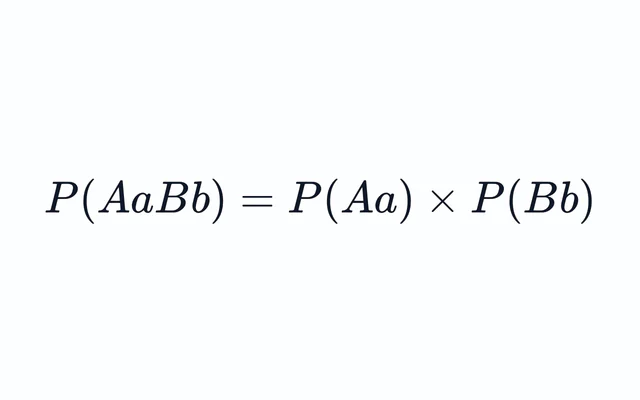
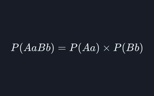
- Random mating: built in here, so the genotype counts only scatter around p², 2pq and q².
- No natural selection: pick a preset other than Neutral, or Custom fitnesses that differ.
Predictions: heterozygosity H₀(1 − 1/2N)ᵗ under drift alone (Coop eq 4.2); fixation probability (1 − e^(−2Nsp))/(1 − e^(−2Ns)) for weak additive selection, s ≪ 1 (eq 12.11), shown up to |s| = 0.1; pₑ = s₂/(s₁ + s₂) under heterozygote advantage (Coop 10.1.1).
Cite this tool
Citing this tool
Last updated . Add the date you accessed it as well, which a citation of a page that can change asks for. If a specific result matters, cite the permalink from the tool’s share row instead of this page: it reproduces the exact parameters.
The equation
Coop, Population and Quantitative Genetics (UC Davis, 2021), chapters 4, 10, 11 and 12
What the simulator shows
Each line is one population of N individuals, tracked at a single gene with two alleles, A at frequency p and a at q = 1 − p. Every generation the N offspring draw their two gene copies at random from the parents’ gametes, so the number of A copies is a binomial sample of size 2N. That chance sampling is genetic drift, a change in allele frequencies from a nonselective process in a small population (AP Biology 7.4.A.1). Run 10 populations from the same start and they wander apart; some lose A, some fix it, and the dashed curve shows where a population with no drift would be.
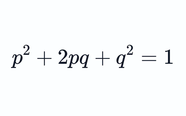
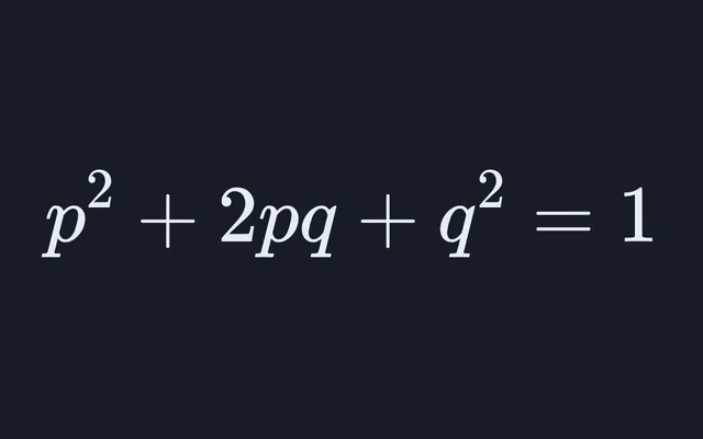
Under the plot, the strip shows the selected population’s genotypes at the cursor, one dot per individual up to 200 and one per percent above that: AA filled, aa hollow and Aa half of each. The readouts set the observed genotype shares beside the Hardy-Weinberg expectations p², 2pq and q² at the same p, the numbers the Hardy-Weinberg calculator works out.
What to try
- Drift alone. The opening run: N = 50, 10 populations, p₀ = 0.5, neutral. Heterozygosity falls by a factor 1 − 1/2N = 0.99 a generation, so after 50 generations the expected 2pq is 0.99⁵⁰ = 0.605 of where it started, and after 200 generations 0.134 (Coop eq 4.2). The plot under the stage draws that curve against the mean of the populations.
- A bigger population. Set N to 500 and the lines spread more slowly: after 200 generations 0.999²⁰⁰ = 0.819 of the heterozygosity is left, against 0.134 at N = 50, and hardly any population fixes or loses A.
- A bottleneck. Choose Bottleneck with 5 individuals for 5 generations. Each of those generations keeps 1 − 1/10 of the heterozygosity, so the bottleneck costs a factor of 0.9⁵ = 0.590, as much as about 52 generations at N = 50.
- Founders. Choose Found a new population with 5 founders. They carry 10 gene copies, so from a parent at p = 0.5 the founders’ frequency has a standard deviation of √(0.25/10) = 0.158, and 2 × 0.5¹⁰ = 0.002 of the time one allele is left behind altogether.
- Selection against drift. Pick Additive with s = 0.02. At N = 10, Ns = 0.2 and the lines look much as they do with no selection; at N = 500, Ns = 10 and almost every population climbs. Coop puts the line at |Ns| ≫ 1 for selection to dominate and |Ns| ≪ 1 for drift.
- Heterozygote advantage. The preset’s fitnesses are 0.9, 1 and 0.85, Coop’s Figure 10.10. With s₁ = 0.1 and s₂ = 0.15 the equilibrium is pₑ = 0.15/0.25 = 0.6, and selection pulls p there from either end.
- Gene flow. Set m to 0.05. With nothing else acting, the gap to the source shrinks by 5 percent a generation, as 0.95ᵗ, so after 14 generations 0.95¹⁴ = 0.488 of it is left.
One generation, step by step
The model is the Wright-Fisher model as Graham Coop’s population genetics notes set it out. It takes the deterministic change first and then samples, in this order:
- Mutation: p(1 − u) + (1 − p)v, with u the rate from A to a and v from a to A.
- Gene flow: (1 − m)p + m·p_M, a share m of the gene pool from a source at p_M.
- Selection on zygotes formed in Hardy-Weinberg proportions: pₛ = (wAA p² + wAa pq) / w̄, with w̄ = wAA p² + 2wAa pq + waa q² (Coop eq 10.18), the same change as Δp = pq(w1 − w2)/w̄ with marginal fitnesses w1 = wAA p + wAa q and w2 = wAa p + waa q (eq 10.23).
- Drift: N offspring, each drawing two copies at frequency pₛ, so the A count k is Binomial(2N, pₛ) and the new p is k/2N. Infinite population skips this step.
The directional presets use Coop’s fitnesses wAA = 1, wAa = 1 − hs, waa = 1 − s: Additive is h = ½, A dominant is h = 0 and A recessive is h = 1. The fixation readout uses eq 12.11, (1 − e^(−2Nsp))/(1 − e^(−2Ns)), which Coop derives for weak additive selection (s ≪ 1) at a constant N, so the readout shows it only up to |s| = 0.1. For an allele with s = 0.02 in a population of 50, starting at p = 0.1, eq 12.11 gives (1 − e^(−0.2))/(1 − e^(−2)) = 0.210, where a neutral allele at 0.1 fixes one time in ten.
Each population has its own random stream from the seed, which the share link carries after the #, so the link replays the same runs. New seed draws a fresh set.
The Hardy-Weinberg conditions
AP Biology 7.5.A.1 lists five conditions for Hardy-Weinberg equilibrium: a large population, no migration, no new mutations, random mating and no natural selection, and says they are never met but give a valuable null hypothesis. Four of them are controls here. Population size and the events break the first, m the second, u and v the third, and unequal fitnesses the fifth: any preset but Neutral, or Custom once its three fitnesses differ. Mating is always random, which is why the genotype shares only scatter around p², 2pq and q².
Mutation at real rates is too slow to watch. Real rates are about 10⁻⁸ per base pair and 10⁻⁶ to 10⁻⁵ per gene a generation (Coop chs 4, 11 and 12), and they move p by less than 0.005 in 500 generations: from p = 1 at u = 10⁻⁵, p falls to (1 − 10⁻⁵)⁵⁰⁰ = 0.995. The sliders run from 10⁻⁶ to 10⁻² so the effect shows. With no selection or gene flow, mutation brings p to v/(u + v).
What this model leaves out
One gene with two alleles, separate generations that do not overlap, no sexes and a population that is the same size each generation apart from the events. Real populations are smaller in effect than in head count, and Coop treats that as the effective population size. Selection here acts on survival from zygote to adult, and every survivor contributes gametes equally.
Sources
- Graham Coop, Population and Quantitative Genetics, University of California, Davis, updated October 2021, licensed CC BY 3.0: chapter 4 (genetic drift, eqs 4.1 and 4.2), chapter 10 (one-locus selection, eqs 10.18 to 10.26 and 10.31, heterozygote advantage, Figure 10.10), chapter 11 (mutation, migration and selection) and chapter 12 (selection with drift, eqs 12.9 to 12.11).
- College Board, AP Biology Course and Exam Description, effective fall 2025, Unit 7: topics 7.4 (population genetics, 7.4.A.1 and 7.4.B.1) and 7.5 (Hardy-Weinberg equilibrium, 7.5.A.1 and 7.5.A.2).
- Association of American Medical Colleges, What’s on the MCAT Exam?, 2020, content category 1C: genetic drift, bottlenecks and the Hardy-Weinberg principle.
The worked figures on this page come from the same model the simulator runs, and its tests pin it to Coop’s equations. The drawings are this site’s own.
Model and assumptions
The method, what it assumes and how accurate it is
- Method
- Monte Carlo over individual events
- Repeatability
- Random, from a seeded generator. A shared link carries the seed, so it replays the same run, game for game, on any machine.
What it assumes
- One locus with two alleles in a diploid population of N that mates at random, in discrete generations that do not overlap, with no sexes: the Wright-Fisher model of Coop’s notes, chapters 4 and 12.
- Each generation runs in a fixed order: mutation p(1 − u) + (1 − p)v, gene flow (1 − m)p + m·p_M, then selection on zygotes in Hardy-Weinberg proportions, p_s = (wAA p² + wAa pq)/w̄ (Coop eq 10.18).
- Drift draws the N offspring two gene copies each at p_s, so the count of A is exactly Binomial(2N, p_s); the draw is exact inversion from the mode, with no normal approximation. The infinite population skips it.
- Every population draws from its own seeded stream, so the seed in the shared link replays each run, and adding populations leaves the first ones unchanged.
- A bottleneck holds N at N_b for its generations; founders are a single generation of n drawn from the parent, after which the population is N again.
- The heterozygosity and fixation readouts are Coop’s eq 4.2, taken a generation at a time, and eq 12.11, which holds for weak additive selection (s ≪ 1) at a constant N with no mutation or gene flow; the readout shows it only up to |s| = 0.1, where it stays within 0.035 of the exact chance.
Where it stops holding. Real populations, whose effective size is usually far below the head count, whose generations overlap and whose mating is not random; several linked loci, where selection at one drags its neighbors along; and selection on fertility rather than survival. The Hardy-Weinberg Calculator is the right tool there.
Numerical accuracy
No integration error: nothing is integrated. Mutation, gene flow and selection are exact one-generation recursions, and drift draws each population’s gene count exactly from Binomial(2N, pₛ) by inversion, so the only spread is the sampling the model exists to show. Each draw takes one 32-bit number from the seeded generator, which resolves probabilities down to 2⁻³², about 2 × 10⁻¹⁰. With 10 populations the share that fixes is a rough check on the predicted fixation probability: its standard error is √(P(1 − P)/n), about 0.13 for P = 0.21 and n = 10.
Common questions
What is genetic drift?
A change in allele frequencies by chance alone: which individuals happen to breed and which gene copies they pass on. AP Biology defines it as a change in allele frequencies attributable to a nonselective process occurring in small populations. In the Wright-Fisher model each generation’s 2N gene copies are a random sample of the last generation’s, so p moves with a variance of p(1 − p)/2N a generation and no average direction (Coop eq 12.10).
How does population size affect genetic drift?
Smaller populations drift faster. Expected heterozygosity falls by a share 1/2N each generation, Hₜ = H₀(1 − 1/2N)ᵗ (Coop eq 4.2). At N = 50 that is a factor of 0.99 a generation, so 0.605 of the starting heterozygosity is left after 50 generations; at N = 500 the figure is 0.951.
What is the difference between the bottleneck effect and the founder effect?
Both are genetic drift in a small group. In a bottleneck the population itself shrinks to a few individuals for at least one generation; in the founder effect a few individuals leave and start a new population, which carries only the alleles they happened to bring (AP Biology 7.4.A.1). Five individuals for five generations keep 0.9⁵ = 0.590 of the heterozygosity, as much loss as about 52 generations at N = 50.
Can genetic drift beat natural selection?
Yes, when selection is weak for the population’s size. Coop puts the line at |Ns|: well above 1, selection decides an allele’s fate, and well below 1, drift does. An additive allele with s = 0.02 starting at p = 0.1 in a population of 50 fixes with probability about 0.21 (Coop eq 12.11), about twice the 0.1 of a neutral allele, and about 4 times in 5 it is lost though it is favored.
What is heterozygote advantage?
Heterozygotes fitter than either homozygote, which keeps both alleles in the population. With fitnesses 1 − s₁, 1 and 1 − s₂ for AA, Aa and aa, the frequency of A settles at pₑ = s₂/(s₁ + s₂) (Coop 10.1.1). For 0.9, 1 and 0.85 that is 0.15/0.25 = 0.6, reached from either end.
Which Hardy-Weinberg conditions does the simulator break?
AP Biology lists five: a large population, no migration, no new mutations, random mating and no natural selection. Population size and the bottleneck and founder events break the first, the migration rate the second, the mutation rates the third, and unequal fitnesses the fifth: any preset but Neutral, or Custom once its fitnesses differ. Mating is always random here, so the genotype shares scatter around p², 2pq and q².